Template:Analysis of non-homogeneous warranty data
Analysis of Non-Homogeneous Warranty Data
In the previous sections and examples it is important to note that the underlying assumption was that the population was homogeneous. In other words, all sold and returned units were exactly the same, i.e. the same population with no design changes and/or modifications. In many situations, as the product matures, design changes are made to enhance and/or improve the reliability of the product. Obviously, an improved product will exhibit different failure characteristics than its predecessor. To analyze such cases, where the population is non-homogeneous, one needs to extract each homogenous group, fit a life model to each group and then project the expected returns for each group based on the number of units at risk for each specific group.
Using IDs in Weibull++
Weibull++ 7 uses the optional IDs column to differentiate between product versions or different designs (lots). Based on this entry, the data are then automatically separated and the parameters for each lot computed. Based on the computed parameters, failure projections can then be obtained. Note that it is important to realize that the same limitations as discussed previously, with regards to the number of failures that are needed, are also applicable here. In other words, distributions can be automatically fitted to lots that have return (failure) data, whereas if no returns have been experienced yet (either because the units are going to be introduced in the future or because no failures happened yet), the user will be asked to specify the parameters, since they can not be computed. Consequently, subsequent estimation/predictions related to these lots would be based on the user specified parameters. Following is an example that illustrates the use of IDs.
Example 5
A company keeps track of its production and returns. The company uses the `Dates of Failure' format to record the data. For the product in question, three versions (A, B and C) have been produced and put in service.
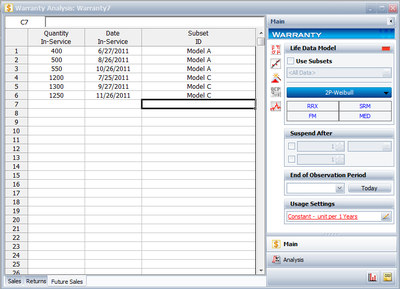
The in-service data is as follows (using the US date format of Month/Day/Year):
Furthermore, the following sales are forecast:
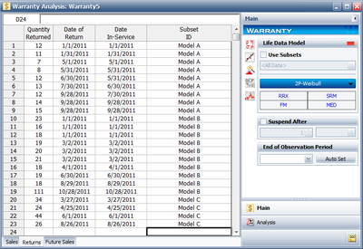
The return data are as follows. Note that in order to identify which lot each unit comes from and be able to compute its time-in-service, each return (failure) includes a return date, the date of when it was put in service and the Model (ID).
Assuming that the above information is as of 5/1/2006, analyze the data using the lognormal as the assumed distribution and MLE as the analysis method, for all models (Model A, Model B, Model C), and provide a return forecast for the next ten months.
Solution to Example 5
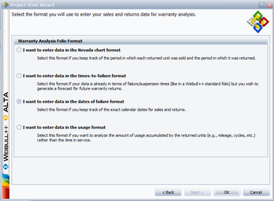
Create a warranty folio by clicking on Project and choosing Add Specialized Folio and then selecting Add Warranty. In the New Warranty Folio Setup window, choose I want to enter data in dates of failure format.
The return data are entered as follows:
The sales data are entered as follows (note that the Use Subsets check box should be checked):
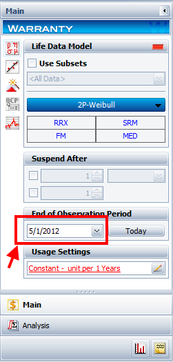
Under the Analysis tab, set the Calculations End Date to (5/1/2006) as shown next:
The calculated parameters, assuming a lognormal distribution and using MLE as the analysis method, are:
Note that in this example, the same distribution type and analysis method were assumed for each of the product models. If desired, different distribution types, analysis methods, confidence bounds methods, etc., can be assumed for each IDs.
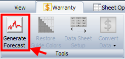
To obtain the expected failures for the next 10 months, click the Generate Forecast button.
- OR:
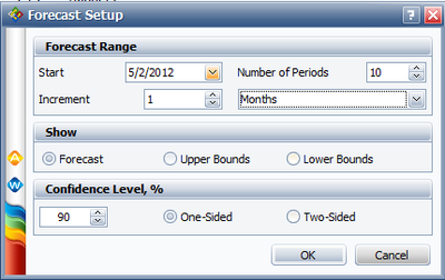
and enter the Start date of 5/2/2006, the Number of Periods as 10, and the Increment number (1) in Months (selected from the drop-down box), as shown next:
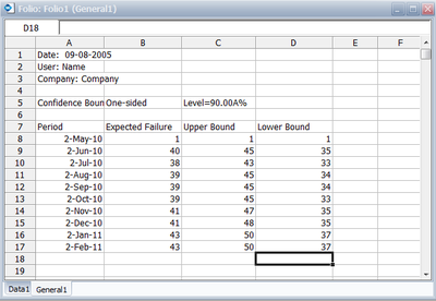
The forecast results are then displayed in a new sheet called Forecast. Part of the forecast table is shown next.
A summary of the analysis can also be obtained by clicking on the Show Analysis Summary (...). The summary of the forecasted returns is as follows:
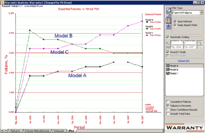
The results can also be seen graphically in the following plot. This is a plot of the expected failures (in percent).
