Template:Crow-amsaa(nhpp)
Crow-AMSAA (NHPP)
In Reliability Analysis for Complex, Repairable Systems (1974), Dr. Larry H. Crow noted that the Duane model could be stochastically represented as a Weibull process, allowing for statistical procedures to be used in the application of this model in reliability growth. This statistical extension became what is known as the Crow-AMSAA (NHPP) model. This method was first developed at the U.S. Army Materiel Systems Analysis Activity (AMSAA). It is frequently used on systems when usage is measured on a continuous scale. It can also be applied for the analysis of one shot items when there is high reliability and large number of trials.
Test programs are generally conducted on a phase by phase basis. The Crow-AMSAA model is designed for tracking the reliability within a test phase and not across test phases. A development testing program may consist of several separate test phases. If corrective actions are introduced during a particular test phase then this type of testing and the associated data are appropriate for analysis by the Crow-AMSAA model. The model analyzes the reliability growth progress within each test phase and can aid in determining the following:
• Reliability of the configuration currently on test
• Reliability of the configuration on test at the end of the test phase
• Expected reliability if the test time for the phase is extended
• Growth rate
• Confidence intervals
• Applicable goodness-of-fit tests
The reliability growth pattern for the Crow-AMSAA model is exactly the same pattern as for the Duane postulate (Chapter 4). That is, the cumulative number of failures is linear when plotted on ln-ln scale. Unlike the Duane postulate, the Crow-AMSAA model is statistically based. Under the Duane postulate, the failure rate is linear on ln-ln scale. However for the Crow-AMSAA model statistical structure, the failure intensity of the underlying non-homogeneous Poisson process (NHPP) is linear when plotted on ln-ln scale. Let [math]\displaystyle{ N(t) }[/math] be the cumulative number of failures observed in cumulative test time [math]\displaystyle{ t }[/math] and let [math]\displaystyle{ \rho (t) }[/math] be the failure intensity for the Crow-AMSAA model. Under the NHPP model, [math]\displaystyle{ \rho (t)\Delta t }[/math] is approximately the probably of a failure occurring over the interval [math]\displaystyle{ [t,t+\Delta t] }[/math] for small [math]\displaystyle{ \Delta t }[/math] . In addition, the expected number of failures experienced over the test interval [math]\displaystyle{ [0,T] }[/math] under the Crow-AMSAA model is given by:
- [math]\displaystyle{ E[N(T)]=\mathop{}_{0}^{T}\rho (t)dt }[/math]
The Crow-AMSAA model assumes that [math]\displaystyle{ \rho (T) }[/math] may be approximated by the Weibull failure rate function:
- [math]\displaystyle{ \rho (T)=\frac{\beta }{{{\eta }^{\beta }}}{{T}^{\beta -1}} }[/math]
Therefore, if [math]\displaystyle{ \lambda =\tfrac{1}{{{\eta }^{\beta }}}, }[/math] the intensity function, [math]\displaystyle{ \rho (T), }[/math] or the instantaneous failure intensity, [math]\displaystyle{ {{\lambda }_{i}}(T) }[/math] , is defined as:
- [math]\displaystyle{ {{\lambda }_{i}}(T)=\lambda \beta {{T}^{\beta -1}},\text{with }T\gt 0,\text{ }\lambda \gt 0\text{ and }\beta \gt 0 }[/math]
In the special case of exponential failure times there is no growth and the failure intensity, [math]\displaystyle{ \rho (t) }[/math] , is equal to [math]\displaystyle{ \lambda }[/math] . In this case, the expected number of failures is given by:
- [math]\displaystyle{ \begin{align} & E[N(T)]= & \mathop{}_{0}^{T}\rho (t)dt \\ & = & \lambda T \end{align} }[/math]
In order for the plot to be linear when plotted on ln-ln scale under the general reliability growth case, the following must hold true where the expected number of failures is equal to:
- [math]\displaystyle{ \begin{align} & E[N(T)]= & \mathop{}_{0}^{T}\rho (t)dt \\ & = & \lambda {{T}^{\beta }} \end{align} }[/math]
To put a statistical structure on the reliability growth process, consider again the special case of no growth. In this case the number of failures, [math]\displaystyle{ N(T), }[/math] experienced during the testing over [math]\displaystyle{ [0,T] }[/math] is random. The expected number of failures, [math]\displaystyle{ N(T), }[/math] is said to follow the homogeneous (constant) Poisson process with mean [math]\displaystyle{ \lambda T }[/math] and is given by:
- [math]\displaystyle{ \underset{}{\overset{}{\mathop{\Pr }}}\,[N(T)=n]=\frac{{{(\lambda T)}^{n}}{{e}^{-\lambda T}}}{n!};\text{ }n=0,1,2,\ldots }[/math]
The Crow-AMSAA generalizes this no growth case to allow for reliability growth due to corrective actions. This generalization keeps the Poisson distribution for the number of failures but allows for the expected number of failures, [math]\displaystyle{ E[N(T)], }[/math] to be linear when plotted on ln-ln scale. The Crow-AMSAA model lets [math]\displaystyle{ E[N(T)]=\lambda {{T}^{\beta }} }[/math] . The probability that the number of failures, [math]\displaystyle{ N(T), }[/math] will be equal to [math]\displaystyle{ n }[/math] under growth is then given by the Poisson distribution:
- [math]\displaystyle{ \underset{}{\overset{}{\mathop{\Pr }}}\,[N(T)=n]=\frac{{{(\lambda {{T}^{\beta }})}^{n}}{{e}^{-\lambda {{T}^{\beta }}}}}{n!};\text{ }n=0,1,2,\ldots }[/math]
This is the general growth situation and the number of failures, [math]\displaystyle{ N(T) }[/math] , follows a non-homogeneous Poisson process. The exponential, "no growth" homogeneous Poisson process is a special case of the non-homogeneous Crow-AMSAA model. This is reflected in the Crow-AMSAA model parameter where [math]\displaystyle{ \beta =1 }[/math] . The cumulative failure rate, [math]\displaystyle{ {{\lambda }_{c}} }[/math] , is:
- [math]\displaystyle{ {{\lambda }_{c}}=\lambda {{T}^{\beta -1}} }[/math]
The cumulative [math]\displaystyle{ MTB{{F}_{c}} }[/math] is:
- [math]\displaystyle{ MTB{{F}_{c}}=\frac{1}{\lambda }{{T}^{1-\beta }} }[/math]
As mentioned above, the local pattern for reliability growth within a test phase is the same as the growth pattern observed by Duane, discussed in Chapter 4. The Duane [math]\displaystyle{ MTB{{F}_{c}} }[/math] is equal to:
- [math]\displaystyle{ MTB{{F}_{{{c}_{DUANE}}}}=b{{T}^{\alpha }} }[/math]
And the Duane cumulative failure rate, [math]\displaystyle{ {{\lambda }_{c}} }[/math] , is:
- [math]\displaystyle{ {{\lambda }_{{{c}_{DUANE}}}}=\frac{1}{b}{{T}^{-\alpha }} }[/math]
Thus a relationship between Crow-AMSAA parameters and Duane parameters can be developed, such that:
- [math]\displaystyle{ \begin{align} & {{b}_{DUANE}}= & \frac{1}{{{\lambda }_{AMSAA}}} \\ & {{\alpha }_{DUANE}}= & 1-{{\beta }_{AMSAA}} \end{align} }[/math]
Note that these relationships are not absolute. They change according to how the parameters (slopes, intercepts, etc.) are defined when the analysis of the data is performed. For the exponential case, [math]\displaystyle{ \beta =1 }[/math] , then [math]\displaystyle{ {{\lambda }_{i}}(T)=\lambda }[/math] , a constant. For [math]\displaystyle{ \beta \gt 1 }[/math] , [math]\displaystyle{ {{\lambda }_{i}}(T) }[/math] is increasing. This indicates a deterioration in system reliability. For [math]\displaystyle{ \beta \lt 1 }[/math] , [math]\displaystyle{ {{\lambda }_{i}}(T) }[/math] is decreasing. This is indicative of reliability growth. Note that the model assumes a Poisson process with Weibull intensity function, not the Weibull distribution. Therefore, statistical procedures for the Weibull distribution do not apply for this model. The parameter [math]\displaystyle{ \lambda }[/math] is called a scale parameter because it depends upon the unit of measurement chosen for [math]\displaystyle{ T }[/math] . [math]\displaystyle{ \beta }[/math] is the shape parameter that characterizes the shape of the graph of the intensity function.
The total number of failures, [math]\displaystyle{ N(T) }[/math] , is a random variable with Poisson distribution. Therefore, the probability that exactly [math]\displaystyle{ n }[/math] failures occur by time [math]\displaystyle{ T }[/math] is:
- [math]\displaystyle{ P[N(T)=n]=\frac{{{[\theta (T)]}^{n}}{{e}^{-\theta (T)}}}{n!} }[/math]
The number of failures occurring in the interval from [math]\displaystyle{ {{T}_{1}} }[/math] to [math]\displaystyle{ {{T}_{2}} }[/math] is a random variable having a Poisson distribution with mean:
- [math]\displaystyle{ \theta ({{T}_{2}})-\theta ({{T}_{1}})=\lambda (T_{2}^{\beta }-T_{1}^{\beta }) }[/math]
The number of failures in any interval is statistically independent of the number of failures in any interval that does not overlap the first interval. At time [math]\displaystyle{ {{T}_{0}} }[/math] , the failure intensity is [math]\displaystyle{ {{\lambda }_{i}}({{T}_{0}})=\lambda \beta T_{0}^{\beta -1} }[/math] . If improvements are not made to the system after time [math]\displaystyle{ {{T}_{0}} }[/math] , it is assumed that failures would continue to occur at the constant rate [math]\displaystyle{ {{\lambda }_{i}}({{T}_{0}})=\lambda \beta T_{0}^{\beta -1} }[/math] . Future failures would then follow an exponential distribution with mean [math]\displaystyle{ m({{T}_{0}})=\tfrac{1}{\lambda \beta T_{0}^{\beta -1}} }[/math] . The instantaneous [math]\displaystyle{ MTBF }[/math] of the system at time [math]\displaystyle{ T }[/math] is:
- [math]\displaystyle{ m(T)=\frac{1}{\lambda \beta {{T}^{\beta -1}}} }[/math]

Dr. Larry H. Crow [17] noted that the Duane Model could be stochastically represented as a Weibull process, allowing for statistical procedures to be used in the application of this model in reliability growth. This statistical extension became what is known as the Crow-AMSAA (NHPP) model. This method was first developed at the U.S. Army Materiel Systems Analysis Activity (AMSAA). It is frequently used on systems when usage is measured on a continuous scale. It can also be applied for the analysis of one shot items when there is high reliability and a large number of trials
Test programs are generally conducted on a phase by phase basis. The Crow-AMSAA model is designed for tracking the reliability within a test phase and not across test phases. A development testing program may consist of several separate test phases. If corrective actions are introduced during a particular test phase, then this type of testing and the associated data are appropriate for analysis by the Crow-AMSAA model. The model analyzes the reliability growth progress within each test phase and can aid in determining the following:
- Reliability of the configuration currently on test
- Reliability of the configuration on test at the end of the test phase
- Expected reliability if the test time for the phase is extended
- Growth rate
- Confidence intervals
- Applicable goodness-of-fit tests
Background
The reliability growth pattern for the Crow-AMSAA model is exactly the same pattern as for the Duane postulate, that is, the cumulative number of failures is linear when plotted on ln-ln scale. Unlike the Duane postulate, the Crow-AMSAA model is statistically based. Under the Duane postulate, the failure rate is linear on ln-ln scale. However, for the Crow-AMSAA model statistical structure, the failure intensity of the underlying non-homogeneous Poisson process (NHPP) is linear when plotted on ln-ln scale.
Let [math]\displaystyle{ N(t)\,\! }[/math] be the cumulative number of failures observed in cumulative test time [math]\displaystyle{ t\,\! }[/math], and let [math]\displaystyle{ \rho (t)\,\! }[/math] be the failure intensity for the Crow-AMSAA model. Under the NHPP model, [math]\displaystyle{ \rho (t)\Delta t\,\! }[/math] is approximately the probably of a failure occurring over the interval [math]\displaystyle{ [t,t+\Delta t]\,\! }[/math] for small [math]\displaystyle{ \Delta t\,\! }[/math]. In addition, the expected number of failures experienced over the test interval [math]\displaystyle{ [0,T]\,\! }[/math] under the Crow-AMSAA model is given by:
- [math]\displaystyle{ E[N(T)]=\int_{0}^{T}\rho (t)dt\,\! }[/math]
The Crow-AMSAA model assumes that [math]\displaystyle{ \rho (T)\,\! }[/math] may be approximated by the Weibull failure rate function:
- [math]\displaystyle{ \rho (T)=\frac{\beta }{{{\eta }^{\beta }}}{{T}^{\beta -1}}\,\! }[/math]
Therefore, if [math]\displaystyle{ \lambda =\tfrac{1}{{{\eta }^{\beta }}},\,\! }[/math] the intensity function, [math]\displaystyle{ \rho (T),\,\! }[/math] or the instantaneous failure intensity, [math]\displaystyle{ {{\lambda }_{i}}(T)\,\! }[/math], is defined as:
- [math]\displaystyle{ {{\lambda }_{i}}(T)=\lambda \beta {{T}^{\beta -1}},\text{with }T\gt 0,\text{ }\lambda \gt 0\text{ and }\beta \gt 0\,\! }[/math]
In the special case of exponential failure times, there is no growth and the failure intensity, [math]\displaystyle{ \rho (t)\,\! }[/math], is equal to [math]\displaystyle{ \lambda \,\! }[/math]. In this case, the expected number of failures is given by:
- [math]\displaystyle{ \begin{align} E[N(T)]= & \int_{0}^{T}\rho (t)dt \\ = & \lambda T \end{align}\,\! }[/math]
In order for the plot to be linear when plotted on ln-ln scale under the general reliability growth case, the following must hold true where the expected number of failures is equal to:
- [math]\displaystyle{ \begin{align} E[N(T)]= & \int_{0}^{T}\rho (t)dt \\ = & \lambda {{T}^{\beta }} \end{align}\,\! }[/math]
To put a statistical structure on the reliability growth process, consider again the special case of no growth. In this case the number of failures, [math]\displaystyle{ N(T),\,\! }[/math] experienced during the testing over [math]\displaystyle{ [0,T]\,\! }[/math] is random. The expected number of failures, [math]\displaystyle{ N(T),\,\! }[/math] is said to follow the homogeneous (constant) Poisson process with mean [math]\displaystyle{ \lambda T\,\! }[/math] and is given by:
- [math]\displaystyle{ \underset{}{\overset{}{\mathop{\Pr }}}\,[N(T)=n]=\frac{{{(\lambda T)}^{n}}{{e}^{-\lambda T}}}{n!};\text{ }n=0,1,2,\ldots \,\! }[/math]
The Crow-AMSAA model generalizes this no growth case to allow for reliability growth due to corrective actions. This generalization keeps the Poisson distribution for the number of failures but allows for the expected number of failures, [math]\displaystyle{ E[N(T)],\,\! }[/math] to be linear when plotted on ln-ln scale. The Crow-AMSAA model lets [math]\displaystyle{ E[N(T)]=\lambda {{T}^{\beta }}\,\! }[/math]. The probability that the number of failures, [math]\displaystyle{ N(T),\,\! }[/math] will be equal to [math]\displaystyle{ n\,\! }[/math] under growth is then given by the Poisson distribution:
- [math]\displaystyle{ \underset{}{\overset{}{\mathop{\Pr }}}\,[N(T)=n]=\frac{{{(\lambda {{T}^{\beta }})}^{n}}{{e}^{-\lambda {{T}^{\beta }}}}}{n!};\text{ }n=0,1,2,\ldots \,\! }[/math]
This is the general growth situation, and the number of failures, [math]\displaystyle{ N(T)\,\! }[/math], follows a non-homogeneous Poisson process. The exponential, "no growth" homogeneous Poisson process is a special case of the non-homogeneous Crow-AMSAA model. This is reflected in the Crow-AMSAA model parameter where [math]\displaystyle{ \beta =1\,\! }[/math]. The cumulative failure rate, [math]\displaystyle{ {{\lambda }_{c}}\,\! }[/math], is:
- [math]\displaystyle{ \begin{align} {{\lambda }_{c}}=\lambda {{T}^{\beta -1}} \end{align}\,\! }[/math]
The cumulative [math]\displaystyle{ MTB{{F}_{c}}\,\! }[/math] is:
- [math]\displaystyle{ MTB{{F}_{c}}=\frac{1}{\lambda }{{T}^{1-\beta }}\,\! }[/math]
As mentioned above, the local pattern for reliability growth within a test phase is the same as the growth pattern observed by Duane. The Duane [math]\displaystyle{ MTB{{F}_{c}}\,\! }[/math] is equal to:
- [math]\displaystyle{ MTB{{F}_{{{c}_{DUANE}}}}=b{{T}^{\alpha }}\,\! }[/math]
And the Duane cumulative failure rate, [math]\displaystyle{ {{\lambda }_{c}}\,\! }[/math], is:
- [math]\displaystyle{ {{\lambda }_{{{c}_{DUANE}}}}=\frac{1}{b}{{T}^{-\alpha }}\,\! }[/math]
Thus a relationship between Crow-AMSAA parameters and Duane parameters can be developed, such that:
- [math]\displaystyle{ \begin{align} {{b}_{DUANE}}= & \frac{1}{{{\lambda }_{AMSAA}}} \\ {{\alpha }_{DUANE}}= & 1-{{\beta }_{AMSAA}} \end{align}\,\! }[/math]
Note that these relationships are not absolute. They change according to how the parameters (slopes, intercepts, etc.) are defined when the analysis of the data is performed. For the exponential case, [math]\displaystyle{ \beta =1\,\! }[/math], then [math]\displaystyle{ {{\lambda }_{i}}(T)=\lambda \,\! }[/math], a constant. For [math]\displaystyle{ \beta \gt 1\,\! }[/math], [math]\displaystyle{ {{\lambda }_{i}}(T)\,\! }[/math] is increasing. This indicates a deterioration in system reliability. For [math]\displaystyle{ \beta \lt 1\,\! }[/math], [math]\displaystyle{ {{\lambda }_{i}}(T)\,\! }[/math] is decreasing. This is indicative of reliability growth. Note that the model assumes a Poisson process with the Weibull intensity function, not the Weibull distribution. Therefore, statistical procedures for the Weibull distribution do not apply for this model. The parameter [math]\displaystyle{ \lambda \,\! }[/math] is called a scale parameter because it depends upon the unit of measurement chosen for [math]\displaystyle{ T\,\! }[/math], while [math]\displaystyle{ \beta \,\! }[/math] is the shape parameter that characterizes the shape of the graph of the intensity function.
The total number of failures, [math]\displaystyle{ N(T)\,\! }[/math], is a random variable with Poisson distribution. Therefore, the probability that exactly [math]\displaystyle{ n\,\! }[/math] failures occur by time [math]\displaystyle{ T\,\! }[/math] is:
- [math]\displaystyle{ P[N(T)=n]=\frac{{{[\theta (T)]}^{n}}{{e}^{-\theta (T)}}}{n!}\,\! }[/math]
The number of failures occurring in the interval from [math]\displaystyle{ {{T}_{1}}\,\! }[/math] to [math]\displaystyle{ {{T}_{2}}\,\! }[/math] is a random variable having a Poisson distribution with mean:
- [math]\displaystyle{ \theta ({{T}_{2}})-\theta ({{T}_{1}})=\lambda (T_{2}^{\beta }-T_{1}^{\beta })\,\! }[/math]
The number of failures in any interval is statistically independent of the number of failures in any interval that does not overlap the first interval. At time [math]\displaystyle{ {{T}_{0}}\,\! }[/math], the failure intensity is [math]\displaystyle{ {{\lambda }_{i}}({{T}_{0}})=\lambda \beta T_{0}^{\beta -1}\,\! }[/math]. If improvements are not made to the system after time [math]\displaystyle{ {{T}_{0}}\,\! }[/math], it is assumed that failures would continue to occur at the constant rate [math]\displaystyle{ {{\lambda }_{i}}({{T}_{0}})=\lambda \beta T_{0}^{\beta -1}\,\! }[/math]. Future failures would then follow an exponential distribution with mean [math]\displaystyle{ m({{T}_{0}})=\tfrac{1}{\lambda \beta T_{0}^{\beta -1}}\,\! }[/math]. The instantaneous MTBF of the system at time [math]\displaystyle{ T\,\! }[/math] is:
- [math]\displaystyle{ m(T)=\frac{1}{\lambda \beta {{T}^{\beta -1}}}\,\! }[/math]
[math]\displaystyle{ m(T)\,\! }[/math] is also called the demonstrated (or achieved) MTBF.
Note About Applicability
The Duane and Crow-AMSAA models are the most frequently used reliability growth models. Their relationship comes from the fact that both make use of the underlying observed linear relationship between the logarithm of cumulative MTBF and cumulative test time. However, the Duane model does not provide a capability to test whether the change in MTBF observed over time is significantly different from what might be seen due to random error between phases. The Crow-AMSAA model allows for such assessments. Also, the Crow-AMSAA allows for development of hypothesis testing procedures to determine growth presence in the data (where [math]\displaystyle{ \beta \lt 1\,\! }[/math] indicates that there is growth in MTBF, [math]\displaystyle{ \beta =1\,\! }[/math] indicates a constant MTBF and [math]\displaystyle{ \beta \gt 1\,\! }[/math] indicates a decreasing MTBF). Additionally, the Crow-AMSAA model views the process of reliability growth as probabilistic, while the Duane model views the process as deterministic.
Failure Times Data
A description of Failure Times Data is presented in the RGA Data Types page.
Parameter Estimation for Failure Times Data
The parameters for the Crow-AMSAA (NHPP) model are estimated using maximum likelihood estimation (MLE). The probability density function (pdf) of the [math]\displaystyle{ {{i}^{th}}\,\! }[/math] event given that the [math]\displaystyle{ {{(i-1)}^{th}}\,\! }[/math] event occurred at [math]\displaystyle{ {{T}_{i-1}}\,\! }[/math] is:
- [math]\displaystyle{ f({{T}_{i}}|{{T}_{i-1}})=\frac{\beta }{\eta }{{\left( \frac{{{T}_{i}}}{\eta } \right)}^{\beta -1}}\cdot {{e}^{-\tfrac{1}{{{\eta }^{\beta }}}\left( T_{i}^{\beta }-T_{i-1}^{\beta } \right)}}\,\! }[/math]
Let [math]\displaystyle{ \lambda =\tfrac{1}{{{\eta }^{\beta }}},\,\! }[/math], the likelihood function is:
- [math]\displaystyle{ L={{\lambda }^{n}}{{\beta }^{n}}{{e}^{-\lambda {{T}^{*\beta }}}}\underset{i=1}{\overset{n}{\mathop \prod }}\,T_{i}^{\beta -1}\,\! }[/math]
where [math]\displaystyle{ {{T}^{*}}\,\! }[/math] is the termination time and is given by:
- [math]\displaystyle{ {{T}^{*}}=\left\{ \begin{matrix} {{T}_{n}}\text{ if the test is failure terminated} \\ T\gt {{T}_{n}}\text{ if the test is time terminated} \\ \end{matrix} \right\}\,\! }[/math]
Taking the natural log on both sides:
- [math]\displaystyle{ \Lambda =n\ln \lambda +n\ln \beta -\lambda {{T}^{*\beta }}+(\beta -1)\underset{i=1}{\overset{n}{\mathop \sum }}\,\ln {{T}_{i}}\,\! }[/math]
And differentiating with respect to [math]\displaystyle{ \lambda \,\! }[/math] yields:
- [math]\displaystyle{ \frac{\partial \Lambda }{\partial \lambda }=\frac{n}{\lambda }-{{T}^{*\beta }}\,\! }[/math]
Set equal to zero and solve for [math]\displaystyle{ \lambda \,\! }[/math] :
- [math]\displaystyle{ \hat{\lambda }=\frac{n}{{{T}^{*\beta }}}\,\! }[/math]
Now differentiate with respect to [math]\displaystyle{ \beta \,\! }[/math] :
- [math]\displaystyle{ \frac{\partial \Lambda }{\partial \beta }=\frac{n}{\beta }-\lambda {{T}^{*\beta }}\ln {{T}^{*}}+\underset{i=1}{\overset{n}{\mathop \sum }}\,\ln {{T}_{i}}\,\! }[/math]
Set equal to zero and solve for [math]\displaystyle{ \beta \,\! }[/math] :
- [math]\displaystyle{ \hat{\beta }=\frac{n}{n\ln {{T}^{*}}-\underset{i=1}{\overset{n}{\mathop{\sum }}}\,\ln {{T}_{i}}}\,\! }[/math]
This equation is used for both failure terminated and time terminated test data.
Biasing and Unbiasing of Beta
The equation above returns the biased estimate, [math]\displaystyle{ \hat{\beta }\,\! }[/math]. The unbiased estimate, [math]\displaystyle{ \bar{\beta }\,\! }[/math], can be calculated by using the following relationships. For time terminated data (the test ends after a specified test time):
- [math]\displaystyle{ \bar{\beta }=\frac{N-1}{N}\hat{\beta }\,\! }[/math]
For failure terminated data (the test ends after a specified number of failures):
- [math]\displaystyle{ \bar{\beta }=\frac{N-2}{N-1}\hat{\beta }\,\! }[/math]
By default [math]\displaystyle{ \hat{\beta }\,\! }[/math] is returned. [math]\displaystyle{ \bar{\beta }\,\! }[/math] can be returned by selecting the Calculate unbiased beta option on the Calculations tab of the Application Setup.
Cramér-von Mises Test
The Cramér-von Mises (CVM) goodness-of-fit test validates the hypothesis that the data follows a non-homogeneous Poisson process with a failure intensity equal to [math]\displaystyle{ u(t)=\lambda \beta {{t}^{\beta -1}}\,\! }[/math]. This test can be applied when the failure data is complete over the continuous interval [math]\displaystyle{ [0,{{T}_{q}}]\,\! }[/math] with no gaps in the data. The CVM data type applies to all data types when the failure times are known, except for Fleet data.
If the individual failure times are known, a Cramér-von Mises statistic is used to test the null hypothesis that a non-homogeneous Poisson process with the failure intensity function [math]\displaystyle{ \rho \left( t \right)=\lambda \,\beta \,{{t}^{\beta -1}}\left( \lambda \gt 0,\beta \gt 0,t\gt 0 \right)\,\! }[/math] properly describes the reliability growth of a system. The Cramér-von Mises goodness-of-fit statistic is then given by the following expression:
- [math]\displaystyle{ C_{M}^{2}=\frac{1}{12M}+\underset{i=1}{\overset{M}{\mathop \sum }}\,{{\left[ {{\left( \frac{{{T}_{i}}}{T} \right)}^{{\bar{\beta }}}}-\frac{2i-1}{2M} \right]}^{2}}\,\! }[/math]
where:
- [math]\displaystyle{ M=\left\{ \begin{matrix} N\text{ if the test is time terminated} \\ N-1\text{ if the test is failure terminated} \\ \end{matrix} \right\}\,\! }[/math]
- [math]\displaystyle{ {\bar{\beta }}\,\! }[/math] is the unbiased value of Beta.
The failure times, [math]\displaystyle{ {{T}_{i}}\,\! }[/math], must be ordered so that [math]\displaystyle{ {{T}_{1}}\lt {{T}_{2}}\lt \ldots \lt {{T}_{M}}\,\! }[/math]. If the statistic [math]\displaystyle{ C_{M}^{2}\,\! }[/math] is less than the critical value corresponding to [math]\displaystyle{ M\,\! }[/math] for a chosen significance level, then you can fail to reject the null hypothesis that the Crow-AMSAA model adequately fits the data.
Critical Values
The following table displays the critical values for the Cramér-von Mises goodness-of-fit test given the sample size, [math]\displaystyle{ M\,\! }[/math], and the significance level, [math]\displaystyle{ \alpha \,\! }[/math].
| Critical values for Cramér-von Mises test | |||||
| [math]\displaystyle{ \alpha \,\! }[/math] | |||||
| [math]\displaystyle{ M\,\! }[/math] | 0.20 | 0.15 | 0.10 | 0.05 | 0.01 |
| 2 | 0.138 | 0.149 | 0.162 | 0.175 | 0.186 |
| 3 | 0.121 | 0.135 | 0.154 | 0.184 | 0.23 |
| 4 | 0.121 | 0.134 | 0.155 | 0.191 | 0.28 |
| 5 | 0.121 | 0.137 | 0.160 | 0.199 | 0.30 |
| 6 | 0.123 | 0.139 | 0.162 | 0.204 | 0.31 |
| 7 | 0.124 | 0.140 | 0.165 | 0.208 | 0.32 |
| 8 | 0.124 | 0.141 | 0.165 | 0.210 | 0.32 |
| 9 | 0.125 | 0.142 | 0.167 | 0.212 | 0.32 |
| 10 | 0.125 | 0.142 | 0.167 | 0.212 | 0.32 |
| 11 | 0.126 | 0.143 | 0.169 | 0.214 | 0.32 |
| 12 | 0.126 | 0.144 | 0.169 | 0.214 | 0.32 |
| 13 | 0.126 | 0.144 | 0.169 | 0.214 | 0.33 |
| 14 | 0.126 | 0.144 | 0.169 | 0.214 | 0.33 |
| 15 | 0.126 | 0.144 | 0.169 | 0.215 | 0.33 |
| 16 | 0.127 | 0.145 | 0.171 | 0.216 | 0.33 |
| 17 | 0.127 | 0.145 | 0.171 | 0.217 | 0.33 |
| 18 | 0.127 | 0.146 | 0.171 | 0.217 | 0.33 |
| 19 | 0.127 | 0.146 | 0.171 | 0.217 | 0.33 |
| 20 | 0.128 | 0.146 | 0.172 | 0.217 | 0.33 |
| 30 | 0.128 | 0.146 | 0.172 | 0.218 | 0.33 |
| 60 | 0.128 | 0.147 | 0.173 | 0.220 | 0.33 |
| 100 | 0.129 | 0.147 | 0.173 | 0.220 | 0.34 |
The significance level represents the probability of rejecting the hypothesis even if it's true. So, there is a risk associated with applying the goodness-of-fit test (i.e., there is a chance that the CVM will indicate that the model does not fit, when in fact it does). As the significance level is increased, the CVM test becomes more stringent. Keep in mind that the CVM test passes when the test statistic is less than the critical value. Therefore, the larger the critical value, the more room there is to work with (e.g., a CVM test with a significance level equal to 0.1 is more strict than a test with 0.01).
Confidence Bounds
The RGA software provides two methods to estimate the confidence bounds for the Crow Extended model when applied to developmental testing data. The Fisher Matrix approach is based on the Fisher Information Matrix and is commonly employed in the reliability field. The Crow bounds were developed by Dr. Larry Crow. See the Crow-AMSAA Confidence Bounds chapter for details on how the confidence bounds are calculated.
Failure Times Data Examples
Example - Parameter Estimation
A prototype of a system was tested with design changes incorporated during the test. The following table presents the data collected over the entire test. Find the Crow-AMSAA parameters and the intensity function using maximum likelihood estimators.
| Row | Time to Event (hr) | [math]\displaystyle{ ln{(T)}\,\! }[/math] |
|---|---|---|
| 1 | 2.7 | 0.99325 |
| 2 | 10.3 | 2.33214 |
| 3 | 12.5 | 2.52573 |
| 4 | 30.6 | 3.42100 |
| 5 | 57.0 | 4.04305 |
| 6 | 61.3 | 4.11578 |
| 7 | 80.0 | 4.38203 |
| 8 | 109.5 | 4.69592 |
| 9 | 125.0 | 4.82831 |
| 10 | 128.6 | 4.85671 |
| 11 | 143.8 | 4.96842 |
| 12 | 167.9 | 5.12337 |
| 13 | 229.2 | 5.43459 |
| 14 | 296.7 | 5.69272 |
| 15 | 320.6 | 5.77019 |
| 16 | 328.2 | 5.79362 |
| 17 | 366.2 | 5.90318 |
| 18 | 396.7 | 5.98318 |
| 19 | 421.1 | 6.04287 |
| 20 | 438.2 | 6.08268 |
| 21 | 501.2 | 6.21701 |
| 22 | 620.0 | 6.42972 |
Solution
For the failure terminated test, [math]\displaystyle{ {\beta}\,\! }[/math] is:
- [math]\displaystyle{ \begin{align} \widehat{\beta }&=\frac{n}{n\ln {{T}^{*}}-\underset{i=1}{\overset{n}{\mathop{\sum }}}\,\ln {{T}_{i}}} \\ &=\frac{22}{22\ln 620-\underset{i=1}{\overset{22}{\mathop{\sum }}}\,\ln {{T}_{i}}} \\ \end{align}\,\! }[/math]
where:
- [math]\displaystyle{ \underset{i=1}{\overset{22}{\mathop \sum }}\,\ln {{T}_{i}}=105.6355\,\! }[/math]
Then:
- [math]\displaystyle{ \widehat{\beta }=\frac{22}{22\ln 620-105.6355}=0.6142\,\! }[/math]
And for [math]\displaystyle{ {\lambda}\,\! }[/math] :
- [math]\displaystyle{ \begin{align} \widehat{\lambda }&=\frac{n}{{{T}^{*\beta }}} \\ & =\frac{22}{{{620}^{0.6142}}}=0.4239 \\ \end{align}\,\! }[/math]
Therefore, [math]\displaystyle{ {{\lambda }_{i}}(T)\,\! }[/math] becomes:
- [math]\displaystyle{ \begin{align} {{\widehat{\lambda }}_{i}}(T)= & 0.4239\cdot 0.6142\cdot {{620}^{-0.3858}} \\ = & 0.0217906\frac{\text{failures}}{\text{hr}} \end{align}\,\! }[/math]
The next figure shows the plot of the failure rate. If no further changes are made, the estimated MTBF is [math]\displaystyle{ \tfrac{1}{0.0217906}\,\! }[/math] or 46 hours.

Example - Confidence Bounds on Failure Intensity
Using the values of [math]\displaystyle{ \hat{\beta }\,\! }[/math] and [math]\displaystyle{ \hat{\lambda }\,\! }[/math] estimated in the example given above, calculate the 90% 2-sided confidence bounds on the cumulative and instantaneous failure intensity.
Solution
Fisher Matrix Bounds
The partial derivatives for the Fisher Matrix confidence bounds are:
- [math]\displaystyle{ \begin{align} \frac{{{\partial }^{2}}\Lambda }{\partial {{\lambda }^{2}}} = & -\frac{22}{{{0.4239}^{2}}}=-122.43 \\ \frac{{{\partial }^{2}}\Lambda }{\partial {{\beta }^{2}}} = & -\frac{22}{{{0.6142}^{2}}}-0.4239\cdot {{620}^{0.6142}}{{(\ln 620)}^{2}}=-967.68 \\ \frac{{{\partial }^{2}}\Lambda }{\partial \lambda \partial \beta } = & -{{620}^{0.6142}}\ln 620=-333.64 \end{align}\,\! }[/math]
The Fisher Matrix then becomes:
- [math]\displaystyle{ \begin{align} \begin{bmatrix}122.43 & 333.64\\ 333.64 & 967.68\end{bmatrix}^{-1} & = \begin{bmatrix}Var(\hat{\lambda}) & Cov(\hat{\beta},\hat{\lambda})\\ Cov(\hat{\beta},\hat{\lambda}) & Var(\hat{\beta})\end{bmatrix} \\ & = \begin{bmatrix} 0.13519969 & -0.046614609\\ -0.046614609 & 0.017105343 \end{bmatrix} \end{align}\,\! }[/math]
For [math]\displaystyle{ T=620\,\! }[/math] hours, the partial derivatives of the cumulative and instantaneous failure intensities are:
- [math]\displaystyle{ \begin{align} \frac{\partial {{\lambda }_{c}}(T)}{\partial \beta }= & \hat{\lambda }{{T}^{\hat{\beta }-1}}\ln (T) \\ = & 0.4239\cdot {{620}^{-0.3858}}\ln 620 \\ = & 0.22811336 \\ \frac{\partial {{\lambda }_{c}}(T)}{\partial \lambda }= & {{T}^{\hat{\beta }-1}} \\ = & {{620}^{-0.3858}} \\ = & 0.083694185 \end{align}\,\! }[/math]
- [math]\displaystyle{ \begin{align} \frac{\partial {{\lambda }_{i}}(T)}{\partial \beta }= & \hat{\lambda }{{T}^{\hat{\beta }-1}}+\hat{\lambda }\hat{\beta }{{T}^{\hat{\beta }-1}}\ln T \\ = & 0.4239\cdot {{620}^{-0.3858}}+0.4239\cdot 0.6142\cdot {{620}^{-0.3858}}\ln 620 \\ = & 0.17558519 \end{align}\,\! }[/math]
- [math]\displaystyle{ \begin{align} \frac{\partial {{\lambda }_{i}}(T)}{\partial \lambda }= & \hat{\beta }{{T}^{\hat{\beta }-1}} \\ = & 0.6142\cdot {{620}^{-0.3858}} \\ = & 0.051404969 \end{align}\,\! }[/math]
Therefore, the variances become:
- [math]\displaystyle{ \begin{align} Var(\hat{\lambda_{c}}(T)) & = 0.22811336^{2}\cdot 0.017105343\ + 0.083694185^{2} \cdot 0.13519969\ -2\cdot 0.22811336\cdot 0.083694185\cdot 0.046614609 \\ & = 0.00005721408 \\ Var(\hat{\lambda_{i}}(T)) & = 0.17558519^{2}\cdot 0.01715343\ + 0.051404969^{2}\cdot 0.13519969\ -2\cdot 0.17558519\cdot 0.051404969\cdot 0.046614609 \\ &= 0.0000431393 \end{align}\,\! }[/math]
The cumulative and instantaneous failure intensities at [math]\displaystyle{ T=620\,\! }[/math] hours are:
- [math]\displaystyle{ \begin{align} {{\lambda }_{c}}(T)= & 0.03548 \\ {{\lambda }_{i}}(T)= & 0.02179 \end{align}\,\! }[/math]
So, at the 90% confidence level and for [math]\displaystyle{ T=620\,\! }[/math] hours, the Fisher Matrix confidence bounds for the cumulative failure intensity are:
- [math]\displaystyle{ \begin{align} {{[{{\lambda }_{c}}(T)]}_{L}}= & 0.02499 \\ {{[{{\lambda }_{c}}(T)]}_{U}}= & 0.05039 \end{align}\,\! }[/math]
The confidence bounds for the instantaneous failure intensity are:
- [math]\displaystyle{ \begin{align} {{[{{\lambda }_{i}}(T)]}_{L}}= & 0.01327 \\ {{[{{\lambda }_{i}}(T)]}_{U}}= & 0.03579 \end{align}\,\! }[/math]
The following figures display plots of the Fisher Matrix confidence bounds for the cumulative and instantaneous failure intensity, respectively.


Crow Bounds
Given that the data is failure terminated, the Crow confidence bounds for the cumulative failure intensity at the 90% confidence level and for [math]\displaystyle{ T=620\,\! }[/math] hours are:
- [math]\displaystyle{ \begin{align} {{[{{\lambda }_{c}}(T)]}_{L}} = & \frac{\chi _{\tfrac{\alpha }{2},2N}^{2}}{2\cdot t} \\ = & \frac{29.787476}{2*620} \\ = & 0.02402 \\ {{[{{\lambda }_{c}}(T)]}_{U}} = & \frac{\chi _{1-\tfrac{\alpha }{2},2N}^{2}}{2\cdot t} \\ = & \frac{60.48089}{2*620} \\ = & 0.048775 \end{align}\,\! }[/math]
The Crow confidence bounds for the instantaneous failure intensity at the 90% confidence level and for [math]\displaystyle{ T=620\,\! }[/math] hours are calculated by first estimating the bounds on the instantaneous MTBF. Once these are calculated, take the inverse as shown below. Details on the confidence bounds for instantaneous MTBF are presented here.
- [math]\displaystyle{ \begin{align} {{[{{\lambda }_{i}}(t)]}_{L}} = & \frac{1}{{{[MTB{{F}_{i}}]}_{U}}} \\ = & \frac{1}{MTB{{F}_{i}}\cdot U} \\ = & 0.01179 \end{align}\,\! }[/math]
- [math]\displaystyle{ \begin{align} {{[{{\lambda }_{i}}(t)]}_{U}}= & \frac{1}{{{[MTB{{F}_{i}}]}_{L}}} \\ = & \frac{1}{MTB{{F}_{i}}\cdot L} \\ = & 0.03253 \end{align}\,\! }[/math]
The following figures display plots of the Crow confidence bounds for the cumulative and instantaneous failure intensity, respectively.


Example - Confidence Bounds on MTBF
Calculate the confidence bounds on the cumulative and instantaneous MTBF for the data from the example given above.
Solution
Fisher Matrix Bounds
From the previous example:
- [math]\displaystyle{ \begin{align} Var(\hat{\lambda }) = & 0.13519969 \\ Var(\hat{\beta }) = & 0.017105343 \\ Cov(\hat{\beta },\hat{\lambda }) = & -0.046614609 \end{align}\,\! }[/math]
And for [math]\displaystyle{ T=620\,\! }[/math] hours, the partial derivatives of the cumulative and instantaneous MTBF are:
- [math]\displaystyle{ \begin{align} \frac{\partial {{m}_{c}}(T)}{\partial \beta }= & -\frac{1}{\hat{\lambda }}{{T}^{1-\hat{\beta }}}\ln T \\ = & -\frac{1}{0.4239}{{620}^{0.3858}}\ln 620 \\ = & -181.23135 \\ \frac{\partial {{m}_{c}}(T)}{\partial \lambda } = & -\frac{1}{{{\hat{\lambda }}^{2}}}{{T}^{1-\hat{\beta }}} \\ = & -\frac{1}{{{0.4239}^{2}}}{{620}^{0.3858}} \\ = & -66.493299 \\ \frac{\partial {{m}_{i}}(T)}{\partial \beta } = & -\frac{1}{\hat{\lambda }{{\hat{\beta }}^{2}}}{{T}^{1-\beta }}-\frac{1}{\hat{\lambda }\hat{\beta }}{{T}^{1-\hat{\beta }}}\ln T \\ = & -\frac{1}{0.4239\cdot {{0.6142}^{2}}}{{620}^{0.3858}}-\frac{1}{0.4239\cdot 0.6142}{{620}^{0.3858}}\ln 620 \\ = & -369.78634 \\ \frac{\partial {{m}_{i}}(T)}{\partial \lambda } = & -\frac{1}{{{\hat{\lambda }}^{2}}\hat{\beta }}{{T}^{1-\hat{\beta }}} \\ = & -\frac{1}{{{0.4239}^{2}}\cdot 0.6142}\cdot {{620}^{0.3858}} \\ = & -108.26001 \end{align}\,\! }[/math]
Therefore, the variances become:
- [math]\displaystyle{ \begin{align} Var({{\hat{m}}_{c}}(T)) = & {{\left( -181.23135 \right)}^{2}}\cdot 0.017105343+{{\left( -66.493299 \right)}^{2}}\cdot 0.13519969 \\ & -2\cdot \left( -181.23135 \right)\cdot \left( -66.493299 \right)\cdot 0.046614609 \\ = & 36.113376 \end{align}\,\! }[/math]
- [math]\displaystyle{ \begin{align} Var({{\hat{m}}_{i}}(T)) = & {{\left( -369.78634 \right)}^{2}}\cdot 0.017105343+{{\left( -108.26001 \right)}^{2}}\cdot 0.13519969 \\ & -2\cdot \left( -369.78634 \right)\cdot \left( -108.26001 \right)\cdot 0.046614609 \\ = & 191.33709 \end{align}\,\! }[/math]
So, at 90% confidence level and [math]\displaystyle{ T=620\,\! }[/math] hours, the Fisher Matrix confidence bounds are:
- [math]\displaystyle{ \begin{align} {{[{{m}_{c}}(T)]}_{L}} = & {{{\hat{m}}}_{c}}(t){{e}^{-{{z}_{\alpha }}\sqrt{Var({{{\hat{m}}}_{c}}(t))}/{{{\hat{m}}}_{c}}(t)}} \\ = & 19.84581 \\ {{[{{m}_{c}}(T)]}_{U}} = & {{{\hat{m}}}_{c}}(t){{e}^{{{z}_{\alpha }}\sqrt{Var({{{\hat{m}}}_{c}}(t))}/{{{\hat{m}}}_{c}}(t)}} \\ = & 40.01927 \end{align}\,\! }[/math]
- [math]\displaystyle{ \begin{align} {{[{{m}_{i}}(T)]}_{L}} = & {{{\hat{m}}}_{i}}(t){{e}^{-{{z}_{\alpha }}\sqrt{Var({{{\hat{m}}}_{i}}(t))}/{{{\hat{m}}}_{i}}(t)}} \\ = & 27.94261 \\ {{[{{m}_{i}}(T)]}_{U}} = & {{{\hat{m}}}_{i}}(t){{e}^{{{z}_{\alpha }}\sqrt{Var({{{\hat{m}}}_{i}}(t))}/{{{\hat{m}}}_{i}}(t)}} \\ = & 75.34193 \end{align}\,\! }[/math]
The following two figures show plots of the Fisher Matrix confidence bounds for the cumulative and instantaneous MTBFs.


Crow Bounds
The Crow confidence bounds for the cumulative MTBF and the instantaneous MTBF at the 90% confidence level and for [math]\displaystyle{ T=620\,\! }[/math] hours are:
- [math]\displaystyle{ \begin{align} {{[{{m}_{c}}(T)]}_{L}} = & \frac{1}{{{[{{\lambda }_{c}}(T)]}_{U}}} \\ = & 20.5023 \\ {{[{{m}_{c}}(T)]}_{U}} = & \frac{1}{{{[{{\lambda }_{c}}(T)]}_{L}}} \\ = & 41.6282 \end{align}\,\! }[/math]
- [math]\displaystyle{ \begin{align} {{[MTB{{F}_{i}}]}_{L}} = & MTB{{F}_{i}}\cdot {{\Pi }_{1}} \\ = & 30.7445 \\ {{[MTB{{F}_{i}}]}_{U}} = & MTB{{F}_{i}}\cdot {{\Pi }_{2}} \\ = & 84.7972 \end{align}\,\! }[/math]
The figures below show plots of the Crow confidence bounds for the cumulative and instantaneous MTBF.


Confidence bounds can also be obtained on the parameters [math]\displaystyle{ \hat{\beta }\,\! }[/math] and [math]\displaystyle{ \hat{\lambda }\,\! }[/math]. For Fisher Matrix confidence bounds:
- [math]\displaystyle{ \begin{align} {{\beta }_{L}} = & \hat{\beta }{{e}^{{{z}_{\alpha }}\sqrt{Var(\hat{\beta })}/\hat{\beta }}} \\ = & 0.4325 \\ {{\beta }_{U}} = & \hat{\beta }{{e}^{-{{z}_{\alpha }}\sqrt{Var(\hat{\beta })}/\hat{\beta }}} \\ = & 0.8722 \end{align}\,\! }[/math]
and:
- [math]\displaystyle{ \begin{align} {{\lambda }_{L}} = & \hat{\lambda }{{e}^{{{z}_{\alpha }}\sqrt{Var(\hat{\lambda })}/\hat{\lambda }}} \\ = & 0.1016 \\ {{\lambda }_{U}} = & \hat{\lambda }{{e}^{-{{z}_{\alpha }}\sqrt{Var(\hat{\lambda })}/\hat{\lambda }}} \\ = & 1.7691 \end{align}\,\! }[/math]
For Crow confidence bounds:
- [math]\displaystyle{ \begin{align} {{\beta }_{L}}= & 0.4527 \\ {{\beta }_{U}}= & 0.9350 \end{align}\,\! }[/math]
and:
- [math]\displaystyle{ \begin{align} {{\lambda }_{L}}= & 0.2870 \\ {{\lambda }_{U}}= & 0.5827 \end{align}\,\! }[/math]
Multiple Systems
When more than one system is placed on test during developmental testing, there are multiple data types which are available depending on the testing strategy and the format of the data. The data types that allow for the analysis of multiple systems using the Crow-AMSAA (NHPP) model are given below:
- Multiple Systems (Known Operating Times)
- Multiple Systems (Concurrent Operating Times)
- Multiple Systems with Dates
Goodness-of-fit Tests
For all multiple systems data types, the Cramér-von Mises (CVM) Test is available. For Multiple Systems (Concurrent Operating Times) and Multiple Systems with Dates, two additional tests are also available: Laplace Trend Test and Common Beta Hypothesis.
Multiple Systems (Known Operating Times)
A description of Multiple Systems (Known Operating Times) is presented on the RGA Data Types page.
Consider the data in the table below for two prototypes that were placed in a reliability growth test.
| Failure Number | Failed Unit | Test Time Unit 1 (hr) | Test Time Unit 2 (hr) | Total Test Time (hr) | [math]\displaystyle{ ln{(T)}\,\! }[/math] |
|---|---|---|---|---|---|
| 1 | 1 | 1.0 | 1.7 | 2.7 | 0.99325 |
| 2 | 1 | 7.3 | 3.0 | 10.3 | 2.33214 |
| 3 | 2 | 8.7 | 3.8 | 12.5 | 2.52573 |
| 4 | 2 | 23.3 | 7.3 | 30.6 | 3.42100 |
| 5 | 2 | 46.4 | 10.6 | 57.0 | 4.04305 |
| 6 | 1 | 50.1 | 11.2 | 61.3 | 4.11578 |
| 7 | 1 | 57.8 | 22.2 | 80.0 | 4.38203 |
| 8 | 2 | 82.1 | 27.4 | 109.5 | 4.69592 |
| 9 | 2 | 86.6 | 38.4 | 125.0 | 4.82831 |
| 10 | 1 | 87.0 | 41.6 | 128.6 | 4.85671 |
| 11 | 2 | 98.7 | 45.1 | 143.8 | 4.96842 |
| 12 | 1 | 102.2 | 65.7 | 167.9 | 5.12337 |
| 13 | 1 | 139.2 | 90.0 | 229.2 | 5.43459 |
| 14 | 1 | 166.6 | 130.1 | 296.7 | 5.69272 |
| 15 | 2 | 180.8 | 139.8 | 320.6 | 5.77019 |
| 16 | 1 | 181.3 | 146.9 | 328.2 | 5.79362 |
| 17 | 2 | 207.9 | 158.3 | 366.2 | 5.90318 |
| 18 | 2 | 209.8 | 186.9 | 396.7 | 5.98318 |
| 19 | 2 | 226.9 | 194.2 | 421.1 | 6.04287 |
| 20 | 1 | 232.2 | 206.0 | 438.2 | 6.08268 |
| 21 | 2 | 267.5 | 233.7 | 501.2 | 6.21701 |
| 22 | 2 | 330.1 | 289.9 | 620.0 | 6.42972 |
The Failed Unit column indicates the system that failed and is meant to be informative, but it does not affect the calculations. To combine the data from both systems, the system ages are added together at the times when a failure occurred. This is seen in the Total Test Time column above. Once the single timeline is generated, then the calculations for the parameters Beta and Lambda are the same as the process presented for Failure Times Data. The results of this analysis would match the results of Failure Times - Example 1.
Multiple Systems (Concurrent Operating Times)
A description of Multiple Systems (Concurrent Operating Times) is presented on the RGA Data Types page.
Parameter Estimation for Multiple Systems (Concurrent Operating Times)
To estimate the parameters, the equivalent system must first be determined. The equivalent single system (ESS) is calculated by summing the usage across all systems when a failure occurs. Keep in mind that Multiple Systems (Concurrent Operating Times) assumes that the systems are running simultaneously and accumulate the same usage. If the systems have different end times then the equivalent system must only account for the systems that are operating when a failure occurred. Systems with a start time greater than zero are shifted back to t = 0. This is the same as having a start time equal to zero and the converted end time is equal to the end time minus the start time. In addition, all failures times are adjusted by subtracting the start time from each value to ensure that all values occur within t = 0 and the adjusted end time. A start time greater than zero indicates that it is not known as to what events occurred at a time less than the start time. This may have been caused by the events during this period not being tracked and/or recorded properly.
As an example, consider two systems have entered a reliability growth test. Both systems have a start time equal to zero and both begin the test with the same configuration. System 1 operated for 100 hours and System 2 operated for 125 hours. The failure times for each system are given below:
- System 1: 25, 47, 80
- System 2: 15, 62, 89, 110
To build the ESS, the total accumulated hours across both systems is taken into account when a failure occurs. Therefore, given the data for Systems 1 and 2, the ESS is comprised of the following events: 30, 50, 94, 124, 160, 178, 210.
The ESS combines the data from both systems into a single timeline. The termination time for the ESS is (100 + 125) = 225 hours. The parameter estimates for [math]\displaystyle{ \hat{\beta }\,\! }[/math] and [math]\displaystyle{ \hat{\lambda}\,\! }[/math] are then calculated using the ESS. This process is the same as the method for Failure Times data.
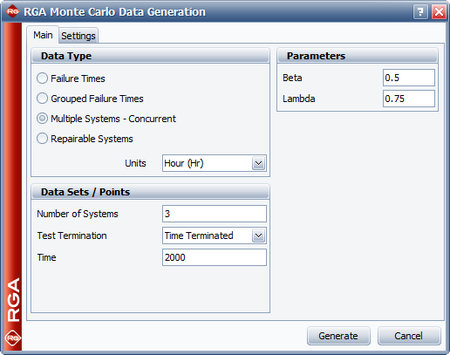
Example - Concurrent Operating Times
Six systems were subjected to a reliability growth test, and a total of 82 failures were observed. Given the data in the table below, which presents the start/end times and times-to-failure for each system, do the following:
- Estimate the parameters of the Crow-AMSAA model using maximum likelihood estimation.
- Determine how many additional failures would be generated if testing continues until 3,000 hours.
| System # | 1 | 2 | 3 | 4 | 5 | 6 |
| Start Time (Hr) | 0 | 0 | 0 | 0 | 0 | 0 |
| End Time (Hr) | 504 | 541 | 454 | 474 | 436 | 500 |
| Failure Times (Hr) | 21 | 83 | 26 | 36 | 23 | 7 |
| 29 | 83 | 26 | 306 | 46 | 13 | |
| 43 | 83 | 57 | 306 | 127 | 13 | |
| 43 | 169 | 64 | 334 | 166 | 31 | |
| 43 | 213 | 169 | 354 | 169 | 31 | |
| 66 | 299 | 213 | 395 | 213 | 82 | |
| 115 | 375 | 231 | 403 | 213 | 109 | |
| 159 | 431 | 231 | 448 | 255 | 137 | |
| 199 | 231 | 456 | 369 | 166 | ||
| 202 | 231 | 461 | 374 | 200 | ||
| 222 | 304 | 380 | 210 | |||
| 248 | 383 | 415 | 220 | |||
| 248 | 301 | |||||
| 255 | 422 | |||||
| 286 | 437 | |||||
| 286 | 469 | |||||
| 304 | 469 | |||||
| 320 | ||||||
| 348 | ||||||
| 364 | ||||||
| 404 | ||||||
| 410 | ||||||
| 429 |
Solution
- To estimate the parameters [math]\displaystyle{ \hat{\beta }\,\! }[/math] and [math]\displaystyle{ \hat{\lambda}\,\! }[/math], the equivalent single system (ESS) must first be determined. The ESS is given below:
Equivalent Single System Row Time to Event (hr) Row Time to Event (hr) Row Time to Event (hr) Row Time to Event (hr) 1 42 22 498 43 1386 64 2214 2 78 23 654 44 1386 65 2244 3 78 24 690 45 1386 66 2250 4 126 25 762 46 1386 67 2280 5 138 26 822 47 1488 68 2298 6 156 27 954 48 1488 69 2370 7 156 28 996 49 1530 70 2418 8 174 29 996 50 1530 71 2424 9 186 30 1014 51 1716 72 2460 10 186 31 1014 52 1716 73 2490 11 216 32 1014 53 1794 74 2532 12 258 33 1194 54 1806 75 2574 13 258 34 1200 55 1824 76 2586 14 258 35 1212 56 1824 77 2621 15 276 36 1260 57 1836 78 2676 16 342 37 1278 58 1836 79 2714 17 384 38 1278 59 1920 80 2734 18 396 39 1278 60 2004 81 2766 19 492 40 1278 61 2088 82 2766 20 498 41 1320 62 2124 21 498 42 1332 63 2184 Given the ESS data, the value of [math]\displaystyle{ \hat{\beta }\,\! }[/math] is calculated using:
- [math]\displaystyle{ \hat{\beta }=\frac{n}{n\ln {{T}^{*}}-\underset{i=1}{\overset{n}{\mathop{\sum }}}\,\ln {{T}_{i}}}\,\! }[/math]
- [math]\displaystyle{ \hat{\beta }=0.8939\,\! }[/math]
where [math]\displaystyle{ n\,\! }[/math] is the number of failures and [math]\displaystyle{ T^*\,\! }[/math] is the termination time. The termination time is the sum of end times for each of the systems, which equals 2,909.
[math]\displaystyle{ \hat{\lambda}\,\! }[/math] is estimated with:
- [math]\displaystyle{ \hat{\lambda }=\frac{n}{{{T}^{*}}^{\beta }} }[/math]
- [math]\displaystyle{ \hat{\lambda }=0.0657\,\! }[/math]
The next figure shows the parameters estimated using RGA.

- The number of failures can be estimated using the Quick Calculation Pad, as shown next. The estimated number of failures at 3,000 hours is equal to 84.2892 and 82 failures were observed during testing. Therefore, the number of additional failures generated if testing continues until 3,000 hours is equal to [math]\displaystyle{ 84.2892-82=2.2892\approx 3\,\! }[/math]

Multiple Systems with Dates
An overview of the Multiple Systems with Dates data type is presented on the RGA Data Types page. While Multiple Systems with Dates requires a date for each event, including the start and end times for each system, once the equivalent single system is determined, the parameter estimation is the same as it is for Multiple Systems (Concurrent Operating Times). See Parameter Estimation for Multiple Systems (Concurrent Operating Times) for details.
Grouped Data
A description of Grouped Data is presented in the RGA Data Types page.
Parameter Estimation for Grouped Data
For analyzing grouped data, we follow the same logic described previously for the Duane model. If the [math]\displaystyle{ E[N(T)]\,\! }[/math] equation from the Background section above is linearized:
- [math]\displaystyle{ \begin{align} \ln [E(N(T))]=\ln \lambda +\beta \ln T \end{align}\,\! }[/math]
According to Crow [9], the likelihood function for the grouped data case, (where [math]\displaystyle{ {{n}_{1}},\,\! }[/math] [math]\displaystyle{ {{n}_{2}},\,\! }[/math] [math]\displaystyle{ {{n}_{3}},\ldots ,\,\! }[/math] [math]\displaystyle{ {{n}_{k}}\,\! }[/math] failures are observed and [math]\displaystyle{ k\,\! }[/math] is the number of groups), is:
- [math]\displaystyle{ \underset{i=1}{\overset{k}{\mathop \prod }}\,\underset{}{\overset{}{\mathop{\Pr }}}\,({{N}_{i}}={{n}_{i}})=\underset{i=1}{\overset{k}{\mathop \prod }}\,\frac{{{(\lambda T_{i}^{\beta }-\lambda T_{i-1}^{\beta })}^{{{n}_{i}}}}\cdot {{e}^{-(\lambda T_{i}^{\beta }-\lambda T_{i-1}^{\beta })}}}{{{n}_{i}}!}\,\! }[/math]
And the MLE of [math]\displaystyle{ \lambda \,\! }[/math] based on this relationship is:
- [math]\displaystyle{ \hat{\lambda }=\frac{n}{T_{k}^{\hat{\beta }}}\,\! }[/math]
where [math]\displaystyle{ n \,\! }[/math] is the total number of failures from all the groups.
The estimate of [math]\displaystyle{ \beta \,\! }[/math] is the value [math]\displaystyle{ \hat{\beta }\,\! }[/math] that satisfies:
- [math]\displaystyle{ \underset{i=1}{\overset{k}{\mathop \sum }}\,{{n}_{i}}\left[ \frac{T_{i}^{\hat{\beta }}\ln {{T}_{i}}-T_{i-1}^{\hat{\beta }}\ln {{T}_{i-1}}}{T_{i}^{\hat{\beta }}-T_{i-1}^{\hat{\beta }}}-\ln {{T}_{k}} \right]=0\,\! }[/math]
See Crow-AMSAA Confidence Bounds for details on how confidence bounds for grouped data are calculated.
Chi-Squared Test
A chi-squared goodness-of-fit test is used to test the null hypothesis that the Crow-AMSAA reliability model adequately represents a set of grouped data. This test is applied only when the data is grouped. The expected number of failures in the interval from [math]\displaystyle{ {{T}_{i-1}}\,\! }[/math] to [math]\displaystyle{ {{T}_{i}}\,\! }[/math] is approximated by:
- [math]\displaystyle{ {{\hat{\theta }}_{i}}=\hat{\lambda }\left( T_{i}^{{\hat{\beta }}}-T_{i-1}^{{\hat{\beta }}} \right)\,\! }[/math]
For each interval, [math]\displaystyle{ {{\hat{\theta }}_{i}}\,\! }[/math] shall not be less than 5 and, if necessary, adjacent intervals may have to be combined so that the expected number of failures in any combined interval is at least 5. Let the number of intervals after this recombination be [math]\displaystyle{ d\,\! }[/math], and let the observed number of failures in the [math]\displaystyle{ {{i}^{th}}\,\! }[/math] new interval be [math]\displaystyle{ {{N}_{i}}\,\! }[/math]. Finally, let the expected number of failures in the [math]\displaystyle{ {{i}^{th}}\,\! }[/math] new interval be [math]\displaystyle{ {{\hat{\theta }}_{i}}\,\! }[/math]. Then the following statistic is approximately distributed as a chi-squared random variable with degrees of freedom [math]\displaystyle{ d-2\,\! }[/math].
- [math]\displaystyle{ {{\chi }^{2}}=\underset{i=1}{\overset{d}{\mathop \sum }}\,\frac{{{({{N}_{i}}-{{\hat{\theta }}_{i}})}^{2}}}{{{\hat{\theta }}_{i}}}\,\! }[/math]
The null hypothesis is rejected if the [math]\displaystyle{ {{\chi }^{2}}\,\! }[/math] statistic exceeds the critical value for a chosen significance level. In this case, the hypothesis that the Crow-AMSAA model adequately fits the grouped data shall be rejected. Critical values for this statistic can be found in chi-squared distribution tables.
Grouped Data Examples
Example - Simple Grouped
Consider the grouped failure times data given in the following table. Solve for the Crow-AMSAA parameters using MLE.
| Run Number | Cumulative Failures | End Time(hours) | [math]\displaystyle{ \ln{(T_i)}\,\! }[/math] | [math]\displaystyle{ \ln{(T_i)^2}\,\! }[/math] | [math]\displaystyle{ \ln{(\theta_i)}\,\! }[/math] | [math]\displaystyle{ \ln{(T_i)}\cdot\ln{(\theta_i)}\,\! }[/math] |
|---|---|---|---|---|---|---|
| 1 | 2 | 200 | 5.298 | 28.072 | 0.693 | 3.673 |
| 2 | 3 | 400 | 5.991 | 35.898 | 1.099 | 6.582 |
| 3 | 4 | 600 | 6.397 | 40.921 | 1.386 | 8.868 |
| 4 | 11 | 3000 | 8.006 | 64.102 | 2.398 | 19.198 |
| Sum = | 25.693 | 168.992 | 5.576 | 38.321 |
Solution
Using RGA, the value of [math]\displaystyle{ \hat{\beta }\,\! }[/math], which must be solved numerically, is 0.6315. Using this value, the estimator of [math]\displaystyle{ \lambda \,\! }[/math] is:
- [math]\displaystyle{ \begin{align} \hat{\lambda } = & \frac{11}{3,{{000}^{0.6315}}} \\ = & 0.0701 \end{align}\,\! }[/math]
Therefore, the intensity function becomes:
- [math]\displaystyle{ \hat{\rho }(T)=0.0701\cdot 0.6315\cdot {{T}^{-0.3685}}\,\! }[/math]
Example - Helicopter System
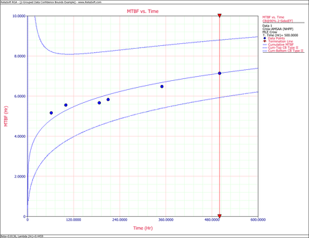
A new helicopter system is under development. System failure data has been collected on five helicopters during the final test phase. The actual failure times cannot be determined since the failures are not discovered until after the helicopters are brought into the maintenance area. However, total flying hours are known when the helicopters are brought in for service, and every 2 weeks each helicopter undergoes a thorough inspection to uncover any failures that may have occurred since the last inspection. Therefore, the cumulative total number of flight hours and the cumulative total number of failures for the 5 helicopters are known for each 2-week period. The total number of flight hours from the test phase is 500, which was accrued over a period of 12 weeks (six 2-week intervals). For each 2-week interval, the total number of flight hours and total number of failures for the 5 helicopters were recorded. The grouped data set is displayed in the following table.
| Interval | Interval Length | Failures in Interval |
|---|---|---|
| 1 | 0 - 62 | 12 |
| 2 | 62 -100 | 6 |
| 3 | 100 - 187 | 15 |
| 4 | 187 - 210 | 3 |
| 5 | 210 - 350 | 18 |
| 6 | 350 - 500 | 16 |
Do the following:
- Estimate the parameters of the Crow-AMSAA model using maximum likelihood estimation.
- Calculate the confidence bounds on the cumulative and instantaneous MTBF using the Fisher Matrix and Crow methods.
Solution
- Using RGA, the value of [math]\displaystyle{ \hat{\beta }\,\! }[/math], must be solved numerically. Once [math]\displaystyle{ \hat{\beta }\,\! }[/math] has been estimated then the value of [math]\displaystyle{ \hat{\lambda }\,\! }[/math] can be determined. The parameter values are displayed below:
- [math]\displaystyle{ \hat{\beta }= 0.81361\,\! }[/math]
- [math]\displaystyle{ \hat{\lambda }= 0.44585\,\! }[/math]
- [math]\displaystyle{ \begin{align} {{\beta }_{L}} = & \hat{\beta }{{e}^{{{z}_{\alpha }}\sqrt{Var(\hat{\beta })}/\hat{\beta }}} \\ = & 0.6546 \\ {{\beta }_{U}} = & \hat{\beta }{{e}^{-{{z}_{\alpha }}\sqrt{Var(\hat{\beta })}/\hat{\beta }}} \\ = & 1.0112 \end{align}\,\! }[/math]
- [math]\displaystyle{ \begin{align} {{\lambda }_{L}} = & \hat{\lambda }{{e}^{{{z}_{\alpha }}\sqrt{Var(\hat{\lambda })}/\hat{\lambda }}} \\ = & 0.14594 \\ {{\lambda }_{U}} = & \hat{\lambda }{{e}^{-{{z}_{\alpha }}\sqrt{Var(\hat{\lambda })}/\hat{\lambda }}} \\ = & 1.36207 \end{align}\,\! }[/math]
- [math]\displaystyle{ \begin{align} {{\beta }_{L}} = & \hat{\beta }(1-S) \\ = & 0.63552 \\ {{\beta }_{U}} = & \hat{\beta }(1+S) \\ = & 0.99170 \end{align}\,\! }[/math]
- [math]\displaystyle{ \begin{align} {{\lambda }_{L}} = & \frac{\chi _{\tfrac{\alpha }{2},2N}^{2}}{2\cdot T_{k}^{\beta }} \\ = & 0.36197 \\ {{\lambda }_{U}} = & \frac{\chi _{1-\tfrac{\alpha }{2},2N+2}^{2}}{2\cdot T_{k}^{\beta }} \\ = & 0.53697 \end{align}\,\! }[/math]
- The Fisher Matrix confidence bounds for the cumulative MTBF and the instantaneous MTBF at the 90% 2-sided confidence level and for [math]\displaystyle{ T=500\,\! }[/math] hour are:
- [math]\displaystyle{ \begin{align} {{[{{m}_{c}}(T)]}_{L}} = & {{{\hat{m}}}_{c}}(t){{e}^{{{z}_{\alpha /2}}\sqrt{Var({{{\hat{m}}}_{c}}(t))}/{{{\hat{m}}}_{c}}(t)}} \\ = & 5.8680 \\ {{[{{m}_{c}}(T)]}_{U}} = & {{{\hat{m}}}_{c}}(t){{e}^{-{{z}_{\alpha /2}}\sqrt{Var({{{\hat{m}}}_{c}}(t))}/{{{\hat{m}}}_{c}}(t)}} \\ = & 8.6947 \end{align}\,\! }[/math]
- [math]\displaystyle{ \begin{align} {{[MTB{{F}_{i}}]}_{L}} = & {{{\hat{m}}}_{i}}(t){{e}^{{{z}_{\alpha /2}}\sqrt{Var({{{\hat{m}}}_{i}}(t))}/{{{\hat{m}}}_{i}}(t)}} \\ = & 6.6483 \\ {{[MTB{{F}_{i}}]}_{U}} = & {{{\hat{m}}}_{i}}(t){{e}^{-{{z}_{\alpha /2}}\sqrt{Var({{{\hat{m}}}_{i}}(t))}/{{{\hat{m}}}_{i}}(t)}} \\ = & 11.5932 \end{align}\,\! }[/math]
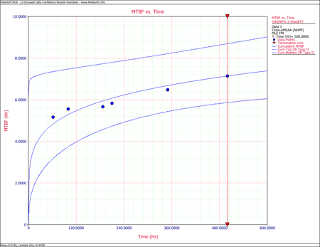
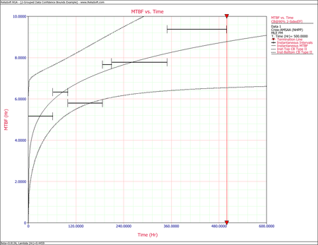
The Crow confidence bounds for the cumulative and instantaneous MTBF at the 90% 2-sided confidence level and for [math]\displaystyle{ T = 500\,\! }[/math]hours are:
- [math]\displaystyle{ \begin{align} {{[{{m}_{c}}(T)]}_{L}} = & \frac{1}{C{{(t)}_{U}}} \\ = & 5.85449 \\ {{[{{m}_{c}}(T)]}_{U}} = & \frac{1}{C{{(t)}_{L}}} \\ = & 8.79822 \end{align}\,\! }[/math]
and:
- [math]\displaystyle{ \begin{align} {{[MTB{{F}_{i}}]}_{L}} = & {{\hat{m}}_{i}}(1-W) \\ = & 6.19623 \\ {{[MTB{{F}_{i}}]}_{U}} = & {{\hat{m}}_{i}}(1+W) \\ = & 11.36223 \end{align}\,\! }[/math]
The next two figures show plots of the Crow confidence bounds for the cumulative and instantaneous MTBF.


Missing Data
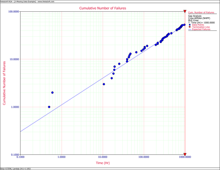
Most of the reliability growth models used for estimating and tracking reliability growth based on test data assume that the data set represents all actual system failure times consistent with a uniform definition of failure (complete data). In practice, this may not always be the case and may result in too few or too many failures being reported over some interval of test time. This may result in distorted estimates of the growth rate and current system reliability. This section discusses a practical reliability growth estimation and analysis procedure based on the assumption that anomalies may exist within the data over some interval of the test period but the remaining failure data follows the Crow-AMSAA reliability growth model. In particular, it is assumed that the beginning and ending points in which the anomalies lie are generated independently of the underlying reliability growth process. The approach for estimating the parameters of the growth model with problem data over some interval of time is basically to not use this failure information. The analysis retains the contribution of the interval to the total test time, but no assumptions are made regarding the actual number of failures over the interval. This is often referred to as gap analysis.
Consider the case where a system is tested for time [math]\displaystyle{ T\,\! }[/math] and the actual failure times are recorded. The time [math]\displaystyle{ T\,\! }[/math] may possibly be an observed failure time. Also, the end points of the gap interval may or may not correspond to a recorded failure time. The underlying assumption is that the data used in the maximum likelihood estimation follows the Crow-AMSAA model with a Weibull intensity function [math]\displaystyle{ \lambda \beta {{t}^{\beta -1}}\,\! }[/math]. It is not assumed that zero failures occurred during the gap interval, rather, it is assumed that the actual number of failures is unknown, and hence no information at all regarding these failure is used to estimate [math]\displaystyle{ \lambda \,\! }[/math] and [math]\displaystyle{ \beta \,\! }[/math].
Let [math]\displaystyle{ {{S}_{1}}\,\! }[/math], [math]\displaystyle{ {{S}_{2}}\,\! }[/math] denote the end points of the gap interval, [math]\displaystyle{ {{S}_{1}}\lt {{S}_{2}}.\,\! }[/math] Let [math]\displaystyle{ 0\lt {{X}_{1}}\lt {{X}_{2}}\lt \ldots \lt {{X}_{{{N}_{1}}}}\le {{S}_{1}}\,\! }[/math] be the failure times over [math]\displaystyle{ (0,\,{{S}_{1}})\,\! }[/math] and let [math]\displaystyle{ {{S}_{2}}\lt {{Y}_{1}}\lt {{Y}_{2}}\lt \ldots \lt {{Y}_{{{N}_{1}}}}\le T\,\! }[/math] be the failure times over [math]\displaystyle{ ({{S}_{2}},\,T)\,\! }[/math]. The maximum likelihood estimates of [math]\displaystyle{ \lambda \,\! }[/math] and [math]\displaystyle{ \beta \,\! }[/math] are values [math]\displaystyle{ \widehat{\lambda }\,\! }[/math] and [math]\displaystyle{ \widehat{\beta }\,\! }[/math] satisfying the following equations.
- [math]\displaystyle{ \widehat{\lambda }=\frac{{{N}_{1}}+{{N}_{2}}}{S\widehat{_{1}^{\beta }}+{{T}^{\widehat{\beta }}}-S_{2}^{\widehat{\beta }}}\,\! }[/math]
- [math]\displaystyle{ \widehat{\beta }=\frac{{{N}_{1}}+{{N}_{2}}}{\widehat{\lambda }\left[ S\widehat{_{1}^{\beta }}\ln {{S}_{1}}+{{T}^{\widehat{\beta }}}\ln T-S_{2}^{\widehat{\beta }}\ln {{S}_{2}} \right]-\left[ \underset{i=1}{\overset{{{N}_{1}}}{\mathop{\sum }}}\,\ln {{X}_{i}}+\underset{i=1}{\overset{{{N}_{2}}}{\mathop{\sum }}}\,\ln {{Y}_{i}} \right]}\,\! }[/math]
In general, these equations cannot be solved explicitly for [math]\displaystyle{ \widehat{\lambda }\,\! }[/math] and [math]\displaystyle{ \widehat{\beta }\,\! }[/math], but must be solved by an iterative procedure.
Example - Gap Analysis
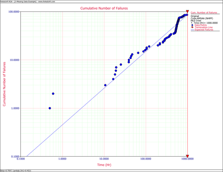
Consider a system under development that was subjected to a reliability growth test for [math]\displaystyle{ T=1,000\,\! }[/math] hours. Each month, the successive failure times, on a cumulative test time basis, were reported. According to the test plan, 125 hours of test time were accumulated on each prototype system each month. The total reliability growth test program lasted for 7 months. One prototype was tested for each of the months 1, 3, 4, 5, 6 and 7 with 125 hours of test time. During the second month, two prototypes were tested for a total of 250 hours of test time. The next table shows the successive [math]\displaystyle{ N=86\,\! }[/math] failure times that were reported for [math]\displaystyle{ T=1,000\,\! }[/math] hours of testing.
| .5 | .6 | 10.7 | 16.6 | 18.3 | 19.2 | 19.5 | 25.3 |
| 39.2 | 39.4 | 43.2 | 44.8 | 47.4 | 65.7 | 88.1 | 97.2 |
| 104.9 | 105.1 | 120.8 | 195.7 | 217.1 | 219 | 257.5 | 260.4 |
| 281.3 | 283.7 | 289.8 | 306.6 | 328.6 | 357.0 | 371.7 | 374.7 |
| 393.2 | 403.2 | 466.5 | 500.9 | 501.5 | 518.4 | 520.7 | 522.7 |
| 524.6 | 526.9 | 527.8 | 533.6 | 536.5 | 542.6 | 543.2 | 545.0 |
| 547.4 | 554.0 | 554.1 | 554.2 | 554.8 | 556.5 | 570.6 | 571.4 |
| 574.9 | 576.8 | 578.8 | 583.4 | 584.9 | 590.6 | 596.1 | 599.1 |
| 600.1 | 602.5 | 613.9 | 616.0 | 616.2 | 617.1 | 621.4 | 622.6 |
| 624.7 | 628.8 | 642.4 | 684.8 | 731.9 | 735.1 | 753.6 | 792.5 |
| 803.7 | 805.4 | 832.5 | 836.2 | 873.2 | 975.1 |
The observed and cumulative number of failures for each month are:
| Month | Time Period | Observed Failure Times | Cumulative Failure Times |
|---|---|---|---|
| 1 | 0-125 | 19 | 19 |
| 2 | 125-375 | 13 | 32 |
| 3 | 375-500 | 3 | 35 |
| 4 | 500-625 | 38 | 73 |
| 5 | 625-750 | 5 | 78 |
| 6 | 750-875 | 7 | 85 |
| 7 | 875-1000 | 1 | 86 |
- Determine the maximum likelihood estimators for the Crow-AMSAA model.
- Evaluate the goodness-of-fit for the model.
- Consider [math]\displaystyle{ (500,\ 625)\,\! }[/math] as the gap interval and determine the maximum likelihood estimates of [math]\displaystyle{ \lambda \,\! }[/math] and [math]\displaystyle{ \beta \,\! }[/math].
Solution
- For the time terminated test:
- [math]\displaystyle{ \begin{align} & \widehat{\beta }= & 0.7597 \\ & \widehat{\lambda }= & 0.4521 \end{align}\,\! }[/math]
- The Cramér-von Mises goodness-of-fit test for this data set yields:
- [math]\displaystyle{ C_{M}^{2}=\tfrac{1}{12M}+\underset{i=1}{\overset{M}{\mathop{\sum }}}\,{{\left[ (\tfrac{{{T}_{i}}}{T})\widehat{^{\beta }}-\tfrac{2i-1}{2M} \right]}^{2}}= 0.6989\,\! }[/math]
Observing the data during the fourth month (between 500 and 625 hours), 38 failures were reported. This number is very high in comparison to the failures reported in the other months. A quick investigation found that a number of new data collectors were assigned to the project during this month. It was also discovered that extensive design changes were made during this period, which involved the removal of a large number of parts. It is possible that these removals, which were not failures, were incorrectly reported as failed parts. Based on knowledge of the system and the test program, it was clear that such a large number of actual system failures was extremely unlikely. The consensus was that this anomaly was due to the failure reporting. For this analysis, it was decided that the actual number of failures over this month is assumed to be unknown, but consistent with the remaining data and the Crow-AMSAA reliability growth model.
- Considering the problem interval [math]\displaystyle{ (500,625)\,\! }[/math] as the gap interval, we will use the data over the interval [math]\displaystyle{ (0,500)\,\! }[/math] and over the interval [math]\displaystyle{ (625,1000).\,\! }[/math] The equations for analyzing missing data are the appropriate equations to estimate [math]\displaystyle{ \lambda \,\! }[/math] and [math]\displaystyle{ \beta \,\! }[/math] because the failure times are known. In this case [math]\displaystyle{ {{S}_{1}}=500,\,{{S}_{2}}=625\,\! }[/math] and [math]\displaystyle{ T=1000,\ {{N}_{1}}=35,\,{{N}_{2}}=13\,\! }[/math]. The maximum likelihood estimates of [math]\displaystyle{ \lambda \,\! }[/math] and [math]\displaystyle{ \beta \,\! }[/math] are:
- [math]\displaystyle{ \begin{align} & \widehat{\beta }= & 0.5596 \\ & \widehat{\lambda }= & 1.1052 \end{align}\,\! }[/math]


Discrete Data
The Crow-AMSAA model can be adapted for the analysis of success/failure data (also called discrete or attribute data). The following discrete data types are available:
- Sequential
- Grouped per Configuration
- Mixed
Sequential data and Grouped per Configuration are very similar as the parameter estimation methodology is the same for both data types. Mixed data is a combination of Sequential Data and Grouped per Configuration and is presented in Mixed Data.
Grouped per Configuration
Suppose system development is represented by [math]\displaystyle{ i\,\! }[/math] configurations. This corresponds to [math]\displaystyle{ i-1\,\! }[/math] configuration changes, unless fixes are applied at the end of the test phase, in which case there would be [math]\displaystyle{ i\,\! }[/math] configuration changes. Let [math]\displaystyle{ {{N}_{i}}\,\! }[/math] be the number of trials during configuration [math]\displaystyle{ i\,\! }[/math] and let [math]\displaystyle{ {{M}_{i}}\,\! }[/math] be the number of failures during configuration [math]\displaystyle{ i\,\! }[/math]. Then the cumulative number of trials through configuration [math]\displaystyle{ i\,\! }[/math], namely [math]\displaystyle{ {{T}_{i}}\,\! }[/math], is the sum of the [math]\displaystyle{ {{N}_{i}}\,\! }[/math] for all [math]\displaystyle{ i\,\! }[/math], or:
- [math]\displaystyle{ {{T}_{i}}=\underset{}{\overset{}{\mathop \sum }}\,{{N}_{i}}\,\! }[/math]
And the cumulative number of failures through configuration [math]\displaystyle{ i\,\! }[/math], namely [math]\displaystyle{ {{K}_{i}}\,\! }[/math], is the sum of the [math]\displaystyle{ {{M}_{i}}\,\! }[/math] for all [math]\displaystyle{ i\,\! }[/math], or:
- [math]\displaystyle{ {{K}_{i}}=\underset{}{\overset{}{\mathop \sum }}\,{{M}_{i}}\,\! }[/math]
The expected value of [math]\displaystyle{ {{K}_{i}}\,\! }[/math] can be expressed as [math]\displaystyle{ E[{{K}_{i}}]\,\! }[/math] and defined as the expected number of failures by the end of configuration [math]\displaystyle{ i\,\! }[/math]. Applying the learning curve property to [math]\displaystyle{ E[{{K}_{i}}]\,\! }[/math] implies:
- [math]\displaystyle{ E\left[ {{K}_{i}} \right]=\lambda T_{i}^{\beta }\,\! }[/math]
Denote [math]\displaystyle{ {{f}_{1}}\,\! }[/math] as the probability of failure for configuration 1 and use it to develop a generalized equation for [math]\displaystyle{ {{f}_{i}}\,\! }[/math] in terms of the [math]\displaystyle{ {{T}_{i}}\,\! }[/math] and [math]\displaystyle{ {{N}_{i}}\,\! }[/math]. From the equation above, the expected number of failures by the end of configuration 1 is:
- [math]\displaystyle{ E\left[ {{K}_{1}} \right]=\lambda T_{1}^{\beta }={{f}_{1}}{{N}_{1}}\,\! }[/math]
- [math]\displaystyle{ \therefore {{f}_{1}}=\frac{\lambda T_{1}^{\beta }}{{{N}_{1}}}\,\! }[/math]
Applying the [math]\displaystyle{ E\left[ {{K}_{i}}\right]\,\! }[/math] equation again and noting that the expected number of failures by the end of configuration 2 is the sum of the expected number of failures in configuration 1 and the expected number of failures in configuration 2:
- [math]\displaystyle{ \begin{align} E\left[ {{K}_{2}} \right] = & \lambda T_{2}^{\beta } \\ = & {{f}_{1}}{{N}_{1}}+{{f}_{2}}{{N}_{2}} \\ = & \lambda T_{1}^{\beta }+{{f}_{2}}{{N}_{2}} \end{align}\,\! }[/math]
- [math]\displaystyle{ \therefore {{f}_{2}}=\frac{\lambda T_{2}^{\beta }-\lambda T_{1}^{\beta }}{{{N}_{2}}}\,\! }[/math]
By this method of inductive reasoning, a generalized equation for the failure probability on a configuration basis, [math]\displaystyle{ {{f}_{i}}\,\! }[/math], is obtained, such that:
- [math]\displaystyle{ {{f}_{i}}=\frac{\lambda T_{i}^{\beta }-\lambda T_{i-1}^{\beta }}{{{N}_{i}}}\,\! }[/math]
In this equation, [math]\displaystyle{ i\,\! }[/math] represents the trial number. Thus, an equation for the reliability (probability of success) for the [math]\displaystyle{ {{i}^{th}}\,\! }[/math] configuration is obtained:
- [math]\displaystyle{ \begin{align} {{R}_{i}}=1-{{f}_{i}} \end{align}\,\! }[/math]
Sequential Data
From the Grouped per Configuration section, the following equation is given:
- [math]\displaystyle{ {{f}_{i}}=\frac{\lambda T_{i}^{\beta }-\lambda T_{i-1}^{\beta }}{{{N}_{i}}}\,\! }[/math]
For the special case where [math]\displaystyle{ {{N}_{i}}=1\,\! }[/math] for all [math]\displaystyle{ i\,\! }[/math], the equation above becomes a smooth curve, [math]\displaystyle{ {{g}_{i}}\,\! }[/math], that represents the probability of failure for trial by trial data, or:
- [math]\displaystyle{ {{g}_{i}}=\lambda \cdot {{i}^{\beta }}-\lambda \cdot {{\left( i-1 \right)}^{\beta }}\,\! }[/math]
When [math]\displaystyle{ {{N}_{i}}=1\,\! }[/math], this is the same as Sequential Data where systems are tested on a trial-by-trial basis. The equation for the reliability for the [math]\displaystyle{ {{i}^{th}}\,\! }[/math] trial is:
- [math]\displaystyle{ \begin{align} {{R}_{i}}=1-{{g}_{i}} \end{align}\,\! }[/math]
Parameter Estimation for Discrete Data
This section describes procedures for estimating the parameters of the Crow-AMSAA model for success/failure data which includes Sequential data and Grouped per Configuration. An example is presented illustrating these concepts. The estimation procedures provide maximum likelihood estimates (MLEs) for the model's two parameters, [math]\displaystyle{ \lambda \,\! }[/math] and [math]\displaystyle{ \beta \,\! }[/math]. The MLEs for [math]\displaystyle{ \lambda \,\! }[/math] and [math]\displaystyle{ \beta \,\! }[/math] allow for point estimates for the probability of failure, given by:
- [math]\displaystyle{ {{\hat{f}}_{i}}=\frac{\hat{\lambda }T_{i}^{{\hat{\beta }}}-\hat{\lambda }T_{i-1}^{{\hat{\beta }}}}{{{N}_{i}}}=\frac{\hat{\lambda }\left( T_{i}^{{\hat{\beta }}}-T_{i-1}^{{\hat{\beta }}} \right)}{{{N}_{i}}}\,\! }[/math]
And the probability of success (reliability) for each configuration [math]\displaystyle{ i\,\! }[/math] is equal to:
- [math]\displaystyle{ {{\hat{R}}_{i}}=1-{{\hat{f}}_{i}}\,\! }[/math]
The likelihood function is:
- [math]\displaystyle{ \underset{i=1}{\overset{k}{\mathop \prod }}\,\left( \begin{matrix} {{N}_{i}} \\ {{M}_{i}} \\ \end{matrix} \right){{\left( \frac{\lambda T_{i}^{\beta }-\lambda T_{i-1}^{\beta }}{{{N}_{i}}} \right)}^{{{M}_{i}}}}{{\left( \frac{{{N}_{i}}-\lambda T_{i}^{\beta }+\lambda T_{i-1}^{\beta }}{{{N}_{i}}} \right)}^{{{N}_{i}}-{{M}_{i}}}}\,\! }[/math]
Taking the natural log on both sides yields:
- [math]\displaystyle{ \begin{align} & \Lambda = & \underset{i=1}{\overset{K}{\mathop \sum }}\,\left[ \ln \left( \begin{matrix} {{N}_{i}} \\ {{M}_{i}} \\ \end{matrix} \right)+{{M}_{i}}\left[ \ln (\lambda T_{i}^{\beta }-\lambda T_{i-1}^{\beta })-\ln {{N}_{i}} \right] \right] \\ & & +\underset{i=1}{\overset{K}{\mathop \sum }}\,\left[ ({{N}_{i}}-{{M}_{i}})\left[ \ln ({{N}_{i}}-\lambda T_{i}^{\beta }+\lambda T_{i-1}^{\beta })-\ln {{N}_{i}} \right] \right] \end{align}\,\! }[/math]
Taking the derivative with respect to [math]\displaystyle{ \lambda \,\! }[/math] and [math]\displaystyle{ \beta \,\! }[/math] respectively, exact MLEs for [math]\displaystyle{ \lambda \,\! }[/math] and [math]\displaystyle{ \beta \,\! }[/math] are values satisfying the following two equations:
- [math]\displaystyle{ \begin{align} & \underset{i=1}{\overset{K}{\mathop \sum }}\,{{H}_{i}}\times {{S}_{i}}= & 0 \\ & \underset{i=1}{\overset{K}{\mathop \sum }}\,{{U}_{i}}\times {{S}_{i}}= & 0 \end{align}\,\! }[/math]
where:
- [math]\displaystyle{ \begin{align} {{H}_{i}}= & \left[ T_{i}^{\beta }\ln {{T}_{i}}-T_{i-1}^{\beta }\ln {{T}_{i-1}} \right] \\ {{S}_{i}}= & \frac{{{M}_{i}}}{\left[ \lambda T_{i}^{\beta }-\lambda T_{i-1}^{\beta } \right]}-\frac{{{N}_{i}}-{{M}_{i}}}{\left[ {{N}_{i}}-\lambda T_{i}^{\beta }+\lambda T_{i-1}^{\beta } \right]} \\ {{U}_{i}}= & T_{i}^{\beta }-T_{i-1}^{\beta }\, \end{align}\,\! }[/math]
Example - Grouped per Configuration
A one-shot system underwent reliability growth development testing for a total of 68 trials. Delayed corrective actions were incorporated after the 14th, 33rd and 48th trials. From trial 49 to trial 68, the configuration was not changed.
- Configuration 1 experienced 5 failures,
- Configuration 2 experienced 3 failures,
- Configuration 3 experienced 4 failures and
- Configuration 4 experienced 4 failures.
Do the following:
- Estimate the parameters of the Crow-AMSAA model using maximum likelihood estimation.
- Estimate the unreliability and reliability by configuration.
Solution
- The parameter estimates for the Crow-AMSAA model using the parameter estimation for discrete data methodology yields [math]\displaystyle{ \lambda = 0.5954\,\! }[/math] and [math]\displaystyle{ \beta =0.7801\,\! }[/math].
- The following table displays the results for probability of failure and reliability, and these results are displayed in the next two plots.
Estimated Failure Probability and Reliability by Configuration Configuration([math]\displaystyle{ i\,\! }[/math]) Estimated Failure Probability Estimated Reliability 1 0.333 0.667 2 0.234 0.766 3 0.206 0.794 4 0.190 0.810 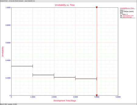


Mixed Data
The Mixed data type provides additional flexibility in terms of how it can handle different testing strategies. Systems can be tested using different configurations in groups or individual trial by trial, or a mixed combination of individual trials and configurations of more than one trial. The Mixed data type allows you to enter the data so that it represents how the systems were tested within the total number of trials. For example, if you launched five (5) missiles for a given configuration and none of them failed during testing, then there would be a row within the data sheet indicating that this configuration operated successfully for these five trials. If the very next trial, the sixth, failed then this would be a separate row within the data. The flexibility with the data entry allows for a greater understanding in terms of how the systems were tested by simply examining the data. The methodology for estimating the parameters [math]\displaystyle{ \hat{\beta }\,\! }[/math] and [math]\displaystyle{ \hat{\lambda}\,\! }[/math] are the same as those presented in the Grouped Data section. With Mixed data, the average reliability and average unreliability within a given interval can also be calculated.
The average unreliability is calculated as:
- [math]\displaystyle{ \text{Average Unreliability }({{t}_{1,}}{{t}_{2}})=\frac{\lambda t_{2}^{\beta }-\lambda t_{1}^{\beta }}{{{t}_{2}}-{{t}_{1}}}\,\! }[/math]
and the average reliability is calculated as:
- [math]\displaystyle{ \text{Average Reliability }({{t}_{1,}}{{t}_{2}})=1-\frac{\lambda t_{2}^{\beta }-\lambda t_{1}^{\beta }}{{{t}_{2}}-{{t}_{1}}}\,\! }[/math]
Mixed Data Confidence Bounds
Bounds on Average Failure Probability
The process to calculate the average unreliability confidence bounds for Mixed data is as follows:
- Calculate the average failure probability [math]\displaystyle{ ({{t}_{1}},{{t}_{2}})\,\! }[/math].
- There will exist a [math]\displaystyle{ {{t}^{*}}\,\! }[/math] between [math]\displaystyle{ {{t}_{1}}\,\! }[/math] and [math]\displaystyle{ {{t}_{2}}\,\! }[/math] such that the instantaneous unreliability at [math]\displaystyle{ {{t}^{*}}\,\! }[/math] equals the average unreliability [math]\displaystyle{ ({{t}_{1}},{{t}_{2}})\,\! }[/math]. The confidence intervals for the instantaneous unreliability at [math]\displaystyle{ {{t}^{*}}\,\! }[/math] are the confidence intervals for the average unreliability [math]\displaystyle{ ({{t}_{1}},{{t}_{2}})\,\! }[/math].
Bounds on Average Reliability
The process to calculate the average reliability confidence bounds for Mixed data is as follows:
- Calculate confidence bounds for average unreliability [math]\displaystyle{ ({{t}_{1}},{{t}_{2}})\,\! }[/math] as described above.
- The confidence bounds for reliability are 1 minus these confidence bounds for average unreliability.
Example - Mixed Data
The table below shows the number of failures of each interval of trials and the cumulative number of trials in each interval for a reliability growth test. For example, the first row indicates that for an interval of 14 trials, 5 failures occurred.
| Failures in Interval | Cumulative Trials |
|---|---|
| 5 | 14 |
| 3 | 33 |
| 4 | 48 |
| 0 | 52 |
| 1 | 53 |
| 0 | 57 |
| 1 | 58 |
| 0 | 62 |
| 1 | 63 |
| 0 | 67 |
| 1 | 68 |
Using the RGA software, the parameters of the Crow-AMSAA model are estimated as follows:
- [math]\displaystyle{ \hat{\beta }=0.7950\,\! }[/math]
and:
- [math]\displaystyle{ \hat{\lambda }=0.5588\,\! }[/math]
As we have seen, the Crow-AMSAA instantaneous failure intensity, [math]\displaystyle{ {{\lambda }_{i}}(T)\,\! }[/math], is defined as:
- [math]\displaystyle{ \begin{align} {{\lambda }_{i}}(T)=\lambda \beta {{T}^{\beta -1}},\text{with }T\gt 0,\text{ }\lambda \gt 0\text{ and }\beta \gt 0 \end{align}\,\! }[/math]
Using the parameter estimates, we can calculate the instantaneous unreliability at the end of the test, or [math]\displaystyle{ T=68.\,\! }[/math]
- [math]\displaystyle{ {{R}_{i}}(68)=0.5588\cdot 0.7950\cdot {{68}^{0.7950-1}}=0.1871\,\! }[/math]
This result that can be obtained from the Quick Calculation Pad (QCP), for [math]\displaystyle{ T=68,\,\! }[/math] as seen in the following picture.

The instantaneous reliability can then be calculated as:
- [math]\displaystyle{ \begin{align} {{R}_{inst}}=1-0.1871=0.8129 \end{align}\,\! }[/math]
Change of Slope
The assumption of the Crow-AMSAA (NHPP) model is that the failure intensity is monotonically increasing, decreasing or remaining constant over time. However, there might be cases in which the system design or the operational environment experiences major changes during the observation period and, therefore, a single model will not be appropriate to describe the failure behavior for the entire timeline. RGA incorporates a methodology that can be applied to scenarios where a major change occurs during a reliability growth test. The test data can be broken into two segments with a separate Crow-AMSAA (NHPP) model applied to each segment.
Consider the data in the following plot from a reliability growth test.

As discussed above, the cumulative number of failures vs. the cumulative time should be linear on logarithmic scales. The next figure shows the data plotted on logarithmic scales.

One can easily recognize that the failure behavior is not constant throughout the duration of the test. Just by observing the data, it can be asserted that a major change occurred at around 140 hours that resulted in a change in the rate of failures. Therefore, using a single model to analyze this data set likely will not be appropriate.
The Change of Slope methodology proposes to split the data into two segments and apply a Crow-AMSAA (NHPP) model to each segment. The time of change that will be used to split the data into the two segments (it will be referred to as [math]\displaystyle{ {{T}_{1}}\,\! }[/math] ) could be estimated just by observing the data, but will most likely be dictated by engineering knowledge of the specific change to the system design or operating conditions. It is important to note that although two separate models will be applied to each segment, the information collected in the first segment (i.e., data up to [math]\displaystyle{ {{T}_{1}}\,\! }[/math] ) will be considered when creating the model for the second segment (i.e., data after [math]\displaystyle{ {{T}_{1}}\,\! }[/math] ). The models presented next can be applied to the reliability growth analysis of a single system or multiple systems.
Model for First Segment (Data up to T1)
The data up to the point of the change that occurs at [math]\displaystyle{ {{T}_{1}}\,\! }[/math] will be analyzed using the Crow-AMSAA (NHPP) model. Based on the ML equations for [math]\displaystyle{ \lambda \,\! }[/math] and [math]\displaystyle{ \beta \,\! }[/math] (in the section Maximum Likelihood Estimators), the ML estimators of the model are:
- [math]\displaystyle{ \widehat{{{\lambda }_{1}}}=\frac{{{n}_{1}}}{T_{1}^{{{\beta }_{1}}}}\,\! }[/math]
and
- [math]\displaystyle{ {{\widehat{\beta }}_{1}}=\frac{{{n}_{1}}}{{{n}_{1}}\ln {{T}_{1}}-\underset{i=1}{\overset{{{n}_{1}}}{\mathop{\sum }}}\,\ln {{t}_{i}}}\,\! }[/math]
where:
- [math]\displaystyle{ {{T}_{1}}\,\! }[/math] is the time when the change occurs
- [math]\displaystyle{ {{n}_{1}}\,\! }[/math] is the number of failures observed up to time [math]\displaystyle{ {{T}_{1}}\,\! }[/math]
- [math]\displaystyle{ {{t}_{i}}\,\! }[/math] is the time at which each corresponding failure was observed
The equation for [math]\displaystyle{ \widehat{\beta_{1}}\,\! }[/math] can be rewritten as follows:
- [math]\displaystyle{ \begin{align} {{\widehat{\beta }}_{1}}= & \frac{{{n}_{1}}}{{{n}_{1}}\ln {{T}_{1}}-\left( \ln {{t}_{1}}+\ln {{t}_{2}}+...+\ln {{t}_{{{n}_{1}}}} \right)} \\ = & \frac{{{n}_{1}}}{(\ln {{T}_{1}}-\ln {{t}_{1}})+(\ln {{T}_{1}}-\ln {{t}_{2}})+(...)+(\ln {{T}_{1}}-\ln {{t}_{{{n}_{1}}}})} \\ = & \frac{{{n}_{1}}}{\ln \tfrac{{{T}_{1}}}{{{t}_{1}}}+\ln \tfrac{{{T}_{1}}}{{{t}_{2}}}+...+\ln \tfrac{{{T}_{1}}}{{{t}_{{{n}_{1}}}}}} \end{align}\,\! }[/math]
or
- [math]\displaystyle{ {{\widehat{\beta }}_{1}}=\frac{{{n}_{1}}}{\underset{i=1}{\overset{{{n}_{1}}}{\mathop{\sum }}}\,\ln \tfrac{{{T}_{1}}}{{{t}_{i}}}}\,\! }[/math]
Model for Second Segment (Data after T1)
The Crow-AMSAA (NHPP) model will be used again to analyze the data after [math]\displaystyle{ {{T}_{1}}\,\! }[/math]. However, the information collected during the first segment will be used when creating the model for the second segment. Given that, the ML estimators of the model parameters in the second segment are:
- [math]\displaystyle{ \widehat{{{\lambda }_{2}}}=\frac{{{n}}}{T_{2}^{{{\beta }_{2}}}}\,\! }[/math]
and:
- [math]\displaystyle{ {{\widehat{\beta }}_{2}}=\frac{{{n}_{2}}}{{{n}_{1}}\ln \tfrac{{{T}_{2}}}{{{T}_{1}}}+\underset{i={{n}_{1}}+1}{\overset{n}{\mathop{\sum }}}\,\ln \tfrac{{{T}_{2}}}{{{t}_{i}}}}\,\! }[/math]
where:
- [math]\displaystyle{ {{n}_{2}}\,\! }[/math] is the number of failures that were observed after [math]\displaystyle{ {{T}_{1}}\,\! }[/math]
- [math]\displaystyle{ n={{n}_{1}}+{{n}_{2}}\,\! }[/math] is the total number of failures observed throughout the test
- [math]\displaystyle{ {{T}_{2}}\,\! }[/math] is the end time of the test. The test can either be failure terminated or time terminated
Example - Multiple MLE
The following table gives the failure times obtained from a reliability growth test of a newly designed system. The test has a duration of 660 hours.
First, apply a single Crow-AMSAA (NHPP) model to all of the data. The following plot shows the expected failures obtained from the model (the line) along with the observed failures (the points).

The plot shows that the model does not seem to accurately track the data. This is confirmed by performing the Cramér-von Mises goodness-of-fit test, which checks the hypothesis that the data follows a non-homogeneous Poisson process with a power law failure intensity. The model fails the goodness-of-fit test because the test statistic (0.3309) is higher than the critical value (0.1729) at the 0.1 significance level. The next figure shows a customized report that displays both the calculated parameters and the statistical test results.

Through further investigation, it is discovered that a significant design change occurred at 400 hours of test time. It is suspected that this modification is responsible for the change in the failure behavior.
In RGA, you have the option to perform a standard Crow-AMSAA (NHPP) analysis, or perform a Change of Slope analysis where you specify a specific breakpoint, as shown in the following figure. RGA actually creates a grouped data set where the data in Segment 1 is included and defined by a single interval to calculate the Segment 2 parameters. However, these results are equivalent to the parameters estimated using the equations presented here.

Therefore, the Change of Slope methodology is applied to break the data into two segments for analysis. The first segment is set from 0 to 400 hours and the second segment is from 401 to 660 hours (which is the end time of the test). The Crow-AMSAA (NHPP) parameters for the first segment (0-400 hours) are:
- [math]\displaystyle{ \widehat{{{\lambda }_{1}}}=\frac{{{n}_{1}}}{T_{1}^{{{\beta }_{1}}}}=\frac{50}{{{400}^{1.0359}}}=0.1008\,\! }[/math]
and
- [math]\displaystyle{ {{\widehat{\beta }}_{1}}=\frac{{{n}_{1}}}{\underset{i=1}{\overset{{{n}_{1}}}{\mathop{\sum }}}\,\ln \tfrac{{{T}_{1}}}{{{t}_{i}}}}=\frac{50}{\underset{i=1}{\overset{50}{\mathop{\sum }}}\,\ln \tfrac{400}{{{t}_{i}}}}=1.0359\,\! }[/math]
The Crow-AMSAA (NHPP) parameters for the second segment (401-660 hours) are:
- [math]\displaystyle{ \widehat{{{\lambda }_{2}}}=\frac{{{n}}}{T_{2}^{{{\beta }_{2}}}}=\frac{58}{{{660}^{0.2971}}}=8.4304\,\! }[/math]
- [math]\displaystyle{ {{\widehat{\beta }}_{2}}=\frac{{{n}_{2}}}{{{n}_{1}}\ln \tfrac{{{T}_{2}}}{{{T}_{1}}}+\underset{i={{n}_{1}}+1}{\overset{n}{\mathop{\sum }}}\,\ln \tfrac{{{T}_{2}}}{{{t}_{i}}}}=\frac{8}{50\ln \tfrac{660}{400}+\underset{i=51}{\overset{58}{\mathop{\sum }}}\,\ln \tfrac{660}{{{T}_{i}}}}=0.2971\,\! }[/math]
The following figure shows a plot of the two-segment analysis along with the observed data. It is obvious that the Change of Slope method tracks the data more accurately.

This can also be verified by performing a chi-squared goodness-of-fit test. The chi-squared statistic is 1.2956, which is lower than the critical value of 12.017 at the 0.1 significance level; therefore, the analysis passes the test. The next figure shows a customized report that displays both the calculated parameters and the statistical test results.

When you have a model that fits the data, it can be used to make accurate predictions and calculations. Metrics such as the demonstrated MTBF at the end of the test or the expected number of failures at later times can be calculated. For example, the following plot shows the instantaneous MTBF vs. time, together with the two-sided 90% confidence bounds. Note that confidence bounds are available for the second segment only. For times up to 400 hours, the parameters of the first segment were used to calculate the MTBF, while the parameters of the second segment were used for times after 400 hours. Also note that the number of failures at the end of segment 1 is not assumed to be equal to the number of failures at the start of segment 2. This can result in a visible jump in the plot, as in this example.

The next figure shows the use of the Quick Calculation Pad (QCP) in the RGA software to calculate the Demonstrated MTBF at the end of the test (instantaneous MTBF at time = 660), together with the two-sided 90% confidence bounds. All the calculations were based on the parameters of the second segment.

More Examples
Determining Whether a Design Meets the MTBF Goal
A prototype of a system was tested at the end of one of its design stages. The test was run for a total of 300 hours and 27 failures were observed. The table below shows the collected data set. The prototype has a design specification of an MTBF equal to 10 hours with a 90% confidence level at 300 hours. Do the following:
- Estimate the parameters of the Crow-AMSAA model using maximum likelihood estimation.
- Does the prototype meet the specified goal?
| 2.6 | 56.5 | 98.1 | 190.7 |
| 16.5 | 63.1 | 101.1 | 193 |
| 16.5 | 70.6 | 132 | 198.7 |
| 17 | 73 | 142.2 | 251.9 |
| 21.4 | 77.7 | 147.7 | 282.5 |
| 29.1 | 93.9 | 149 | 286.1 |
| 33.3 | 95.5 | 167.2 |
Solution
- The next figure shows the parameters estimated using RGA.
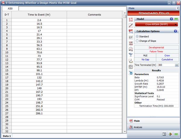
- The instantaneous MTBF with one-sided 90% confidence bounds can be calculated using the Quick Calculation Pad (QCP), as shown next. From the QCP, it is estimated that the lower limit on the MTBF at 300 hours with a 90% confidence level is equal to 10.8170 hours. Therefore, the prototype has met the specified goal.
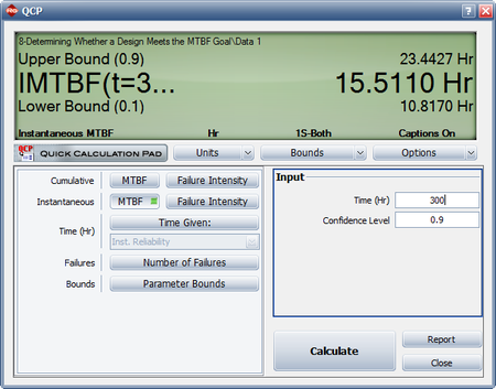


Analyzing Mixed Data for a One-Shot System
A one-shot system underwent reliability growth development for a total of 50 trials. The test was performed as a combination of configuration in groups and individual trial by trial. The table below shows the data set obtained from the test. The first column specifies the number of failures that occurred in each interval, and the second column shows the cumulative number of trials in that interval. Do the following:
- Estimate the parameters of the Crow-AMSAA model using maximum likelihood estimators.
- What are the instantaneous reliability and the 2-sided 90% confidence bounds at the end of the test?
- Plot the cumulative reliability with 2-sided 90% confidence bounds.
- If the test was continued for another 25 trials what would the expected number of additional failures be?
| Failures in Interval | Cumulative Trials | Failures in Interval | Cumulative Trials |
|---|---|---|---|
| 3 | 4 | 1 | 25 |
| 0 | 5 | 1 | 28 |
| 4 | 9 | 0 | 32 |
| 1 | 12 | 2 | 37 |
| 0 | 13 | 0 | 39 |
| 1 | 15 | 1 | 40 |
| 2 | 19 | 1 | 44 |
| 1 | 20 | 0 | 46 |
| 1 | 22 | 1 | 49 |
| 0 | 24 | 0 | 50 |
Solution
- The next figure shows the parameters estimated using RGA.
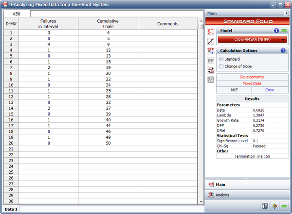
- The figure below shows the calculation of the instantaneous reliability with the 2-sided 90% confidence bounds. From the QCP, it is estimated that the instantaneous reliability at stage 50 (or at the end of the test) is 72.70% with an upper and lower 2-sided 90% confidence bound of 82.36% and 39.59%, respectively.
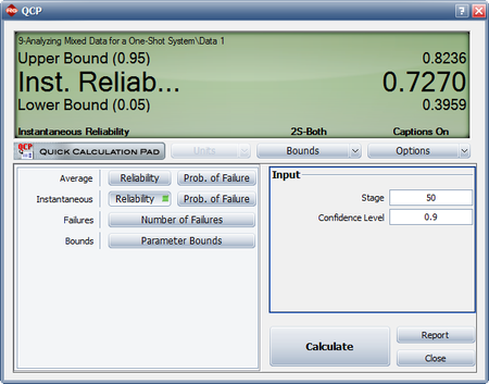
- The following plot shows the cumulative reliability with the 2-sided 90% confidence bounds.
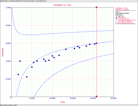
- The last figure shows the calculation of the expected number of failures after 75 trials. From the QCP, it is estimated that the cumulative number of failures after 75 trials is [math]\displaystyle{ 26.3770\approx 27\,\! }[/math]. Since 20 failures occurred in the first 50 trials, the estimated number of additional failures is 7.
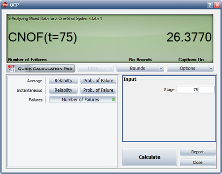


Dr. Larry H. Crow [17] noted that the Duane Model could be stochastically represented as a Weibull process, allowing for statistical procedures to be used in the application of this model in reliability growth. This statistical extension became what is known as the Crow-AMSAA (NHPP) model. This method was first developed at the U.S. Army Materiel Systems Analysis Activity (AMSAA). It is frequently used on systems when usage is measured on a continuous scale. It can also be applied for the analysis of one shot items when there is high reliability and a large number of trials
Test programs are generally conducted on a phase by phase basis. The Crow-AMSAA model is designed for tracking the reliability within a test phase and not across test phases. A development testing program may consist of several separate test phases. If corrective actions are introduced during a particular test phase, then this type of testing and the associated data are appropriate for analysis by the Crow-AMSAA model. The model analyzes the reliability growth progress within each test phase and can aid in determining the following:
- Reliability of the configuration currently on test
- Reliability of the configuration on test at the end of the test phase
- Expected reliability if the test time for the phase is extended
- Growth rate
- Confidence intervals
- Applicable goodness-of-fit tests
Background
The reliability growth pattern for the Crow-AMSAA model is exactly the same pattern as for the Duane postulate, that is, the cumulative number of failures is linear when plotted on ln-ln scale. Unlike the Duane postulate, the Crow-AMSAA model is statistically based. Under the Duane postulate, the failure rate is linear on ln-ln scale. However, for the Crow-AMSAA model statistical structure, the failure intensity of the underlying non-homogeneous Poisson process (NHPP) is linear when plotted on ln-ln scale.
Let [math]\displaystyle{ N(t)\,\! }[/math] be the cumulative number of failures observed in cumulative test time [math]\displaystyle{ t\,\! }[/math], and let [math]\displaystyle{ \rho (t)\,\! }[/math] be the failure intensity for the Crow-AMSAA model. Under the NHPP model, [math]\displaystyle{ \rho (t)\Delta t\,\! }[/math] is approximately the probably of a failure occurring over the interval [math]\displaystyle{ [t,t+\Delta t]\,\! }[/math] for small [math]\displaystyle{ \Delta t\,\! }[/math]. In addition, the expected number of failures experienced over the test interval [math]\displaystyle{ [0,T]\,\! }[/math] under the Crow-AMSAA model is given by:
- [math]\displaystyle{ E[N(T)]=\int_{0}^{T}\rho (t)dt\,\! }[/math]
The Crow-AMSAA model assumes that [math]\displaystyle{ \rho (T)\,\! }[/math] may be approximated by the Weibull failure rate function:
- [math]\displaystyle{ \rho (T)=\frac{\beta }{{{\eta }^{\beta }}}{{T}^{\beta -1}}\,\! }[/math]
Therefore, if [math]\displaystyle{ \lambda =\tfrac{1}{{{\eta }^{\beta }}},\,\! }[/math] the intensity function, [math]\displaystyle{ \rho (T),\,\! }[/math] or the instantaneous failure intensity, [math]\displaystyle{ {{\lambda }_{i}}(T)\,\! }[/math], is defined as:
- [math]\displaystyle{ {{\lambda }_{i}}(T)=\lambda \beta {{T}^{\beta -1}},\text{with }T\gt 0,\text{ }\lambda \gt 0\text{ and }\beta \gt 0\,\! }[/math]
In the special case of exponential failure times, there is no growth and the failure intensity, [math]\displaystyle{ \rho (t)\,\! }[/math], is equal to [math]\displaystyle{ \lambda \,\! }[/math]. In this case, the expected number of failures is given by:
- [math]\displaystyle{ \begin{align} E[N(T)]= & \int_{0}^{T}\rho (t)dt \\ = & \lambda T \end{align}\,\! }[/math]
In order for the plot to be linear when plotted on ln-ln scale under the general reliability growth case, the following must hold true where the expected number of failures is equal to:
- [math]\displaystyle{ \begin{align} E[N(T)]= & \int_{0}^{T}\rho (t)dt \\ = & \lambda {{T}^{\beta }} \end{align}\,\! }[/math]
To put a statistical structure on the reliability growth process, consider again the special case of no growth. In this case the number of failures, [math]\displaystyle{ N(T),\,\! }[/math] experienced during the testing over [math]\displaystyle{ [0,T]\,\! }[/math] is random. The expected number of failures, [math]\displaystyle{ N(T),\,\! }[/math] is said to follow the homogeneous (constant) Poisson process with mean [math]\displaystyle{ \lambda T\,\! }[/math] and is given by:
- [math]\displaystyle{ \underset{}{\overset{}{\mathop{\Pr }}}\,[N(T)=n]=\frac{{{(\lambda T)}^{n}}{{e}^{-\lambda T}}}{n!};\text{ }n=0,1,2,\ldots \,\! }[/math]
The Crow-AMSAA model generalizes this no growth case to allow for reliability growth due to corrective actions. This generalization keeps the Poisson distribution for the number of failures but allows for the expected number of failures, [math]\displaystyle{ E[N(T)],\,\! }[/math] to be linear when plotted on ln-ln scale. The Crow-AMSAA model lets [math]\displaystyle{ E[N(T)]=\lambda {{T}^{\beta }}\,\! }[/math]. The probability that the number of failures, [math]\displaystyle{ N(T),\,\! }[/math] will be equal to [math]\displaystyle{ n\,\! }[/math] under growth is then given by the Poisson distribution:
- [math]\displaystyle{ \underset{}{\overset{}{\mathop{\Pr }}}\,[N(T)=n]=\frac{{{(\lambda {{T}^{\beta }})}^{n}}{{e}^{-\lambda {{T}^{\beta }}}}}{n!};\text{ }n=0,1,2,\ldots \,\! }[/math]
This is the general growth situation, and the number of failures, [math]\displaystyle{ N(T)\,\! }[/math], follows a non-homogeneous Poisson process. The exponential, "no growth" homogeneous Poisson process is a special case of the non-homogeneous Crow-AMSAA model. This is reflected in the Crow-AMSAA model parameter where [math]\displaystyle{ \beta =1\,\! }[/math]. The cumulative failure rate, [math]\displaystyle{ {{\lambda }_{c}}\,\! }[/math], is:
- [math]\displaystyle{ \begin{align} {{\lambda }_{c}}=\lambda {{T}^{\beta -1}} \end{align}\,\! }[/math]
The cumulative [math]\displaystyle{ MTB{{F}_{c}}\,\! }[/math] is:
- [math]\displaystyle{ MTB{{F}_{c}}=\frac{1}{\lambda }{{T}^{1-\beta }}\,\! }[/math]
As mentioned above, the local pattern for reliability growth within a test phase is the same as the growth pattern observed by Duane. The Duane [math]\displaystyle{ MTB{{F}_{c}}\,\! }[/math] is equal to:
- [math]\displaystyle{ MTB{{F}_{{{c}_{DUANE}}}}=b{{T}^{\alpha }}\,\! }[/math]
And the Duane cumulative failure rate, [math]\displaystyle{ {{\lambda }_{c}}\,\! }[/math], is:
- [math]\displaystyle{ {{\lambda }_{{{c}_{DUANE}}}}=\frac{1}{b}{{T}^{-\alpha }}\,\! }[/math]
Thus a relationship between Crow-AMSAA parameters and Duane parameters can be developed, such that:
- [math]\displaystyle{ \begin{align} {{b}_{DUANE}}= & \frac{1}{{{\lambda }_{AMSAA}}} \\ {{\alpha }_{DUANE}}= & 1-{{\beta }_{AMSAA}} \end{align}\,\! }[/math]
Note that these relationships are not absolute. They change according to how the parameters (slopes, intercepts, etc.) are defined when the analysis of the data is performed. For the exponential case, [math]\displaystyle{ \beta =1\,\! }[/math], then [math]\displaystyle{ {{\lambda }_{i}}(T)=\lambda \,\! }[/math], a constant. For [math]\displaystyle{ \beta \gt 1\,\! }[/math], [math]\displaystyle{ {{\lambda }_{i}}(T)\,\! }[/math] is increasing. This indicates a deterioration in system reliability. For [math]\displaystyle{ \beta \lt 1\,\! }[/math], [math]\displaystyle{ {{\lambda }_{i}}(T)\,\! }[/math] is decreasing. This is indicative of reliability growth. Note that the model assumes a Poisson process with the Weibull intensity function, not the Weibull distribution. Therefore, statistical procedures for the Weibull distribution do not apply for this model. The parameter [math]\displaystyle{ \lambda \,\! }[/math] is called a scale parameter because it depends upon the unit of measurement chosen for [math]\displaystyle{ T\,\! }[/math], while [math]\displaystyle{ \beta \,\! }[/math] is the shape parameter that characterizes the shape of the graph of the intensity function.
The total number of failures, [math]\displaystyle{ N(T)\,\! }[/math], is a random variable with Poisson distribution. Therefore, the probability that exactly [math]\displaystyle{ n\,\! }[/math] failures occur by time [math]\displaystyle{ T\,\! }[/math] is:
- [math]\displaystyle{ P[N(T)=n]=\frac{{{[\theta (T)]}^{n}}{{e}^{-\theta (T)}}}{n!}\,\! }[/math]
The number of failures occurring in the interval from [math]\displaystyle{ {{T}_{1}}\,\! }[/math] to [math]\displaystyle{ {{T}_{2}}\,\! }[/math] is a random variable having a Poisson distribution with mean:
- [math]\displaystyle{ \theta ({{T}_{2}})-\theta ({{T}_{1}})=\lambda (T_{2}^{\beta }-T_{1}^{\beta })\,\! }[/math]
The number of failures in any interval is statistically independent of the number of failures in any interval that does not overlap the first interval. At time [math]\displaystyle{ {{T}_{0}}\,\! }[/math], the failure intensity is [math]\displaystyle{ {{\lambda }_{i}}({{T}_{0}})=\lambda \beta T_{0}^{\beta -1}\,\! }[/math]. If improvements are not made to the system after time [math]\displaystyle{ {{T}_{0}}\,\! }[/math], it is assumed that failures would continue to occur at the constant rate [math]\displaystyle{ {{\lambda }_{i}}({{T}_{0}})=\lambda \beta T_{0}^{\beta -1}\,\! }[/math]. Future failures would then follow an exponential distribution with mean [math]\displaystyle{ m({{T}_{0}})=\tfrac{1}{\lambda \beta T_{0}^{\beta -1}}\,\! }[/math]. The instantaneous MTBF of the system at time [math]\displaystyle{ T\,\! }[/math] is:
- [math]\displaystyle{ m(T)=\frac{1}{\lambda \beta {{T}^{\beta -1}}}\,\! }[/math]
[math]\displaystyle{ m(T)\,\! }[/math] is also called the demonstrated (or achieved) MTBF.
Note About Applicability
The Duane and Crow-AMSAA models are the most frequently used reliability growth models. Their relationship comes from the fact that both make use of the underlying observed linear relationship between the logarithm of cumulative MTBF and cumulative test time. However, the Duane model does not provide a capability to test whether the change in MTBF observed over time is significantly different from what might be seen due to random error between phases. The Crow-AMSAA model allows for such assessments. Also, the Crow-AMSAA allows for development of hypothesis testing procedures to determine growth presence in the data (where [math]\displaystyle{ \beta \lt 1\,\! }[/math] indicates that there is growth in MTBF, [math]\displaystyle{ \beta =1\,\! }[/math] indicates a constant MTBF and [math]\displaystyle{ \beta \gt 1\,\! }[/math] indicates a decreasing MTBF). Additionally, the Crow-AMSAA model views the process of reliability growth as probabilistic, while the Duane model views the process as deterministic.
Failure Times Data
A description of Failure Times Data is presented in the RGA Data Types page.
Parameter Estimation for Failure Times Data
The parameters for the Crow-AMSAA (NHPP) model are estimated using maximum likelihood estimation (MLE). The probability density function (pdf) of the [math]\displaystyle{ {{i}^{th}}\,\! }[/math] event given that the [math]\displaystyle{ {{(i-1)}^{th}}\,\! }[/math] event occurred at [math]\displaystyle{ {{T}_{i-1}}\,\! }[/math] is:
- [math]\displaystyle{ f({{T}_{i}}|{{T}_{i-1}})=\frac{\beta }{\eta }{{\left( \frac{{{T}_{i}}}{\eta } \right)}^{\beta -1}}\cdot {{e}^{-\tfrac{1}{{{\eta }^{\beta }}}\left( T_{i}^{\beta }-T_{i-1}^{\beta } \right)}}\,\! }[/math]
Let [math]\displaystyle{ \lambda =\tfrac{1}{{{\eta }^{\beta }}},\,\! }[/math], the likelihood function is:
- [math]\displaystyle{ L={{\lambda }^{n}}{{\beta }^{n}}{{e}^{-\lambda {{T}^{*\beta }}}}\underset{i=1}{\overset{n}{\mathop \prod }}\,T_{i}^{\beta -1}\,\! }[/math]
where [math]\displaystyle{ {{T}^{*}}\,\! }[/math] is the termination time and is given by:
- [math]\displaystyle{ {{T}^{*}}=\left\{ \begin{matrix} {{T}_{n}}\text{ if the test is failure terminated} \\ T\gt {{T}_{n}}\text{ if the test is time terminated} \\ \end{matrix} \right\}\,\! }[/math]
Taking the natural log on both sides:
- [math]\displaystyle{ \Lambda =n\ln \lambda +n\ln \beta -\lambda {{T}^{*\beta }}+(\beta -1)\underset{i=1}{\overset{n}{\mathop \sum }}\,\ln {{T}_{i}}\,\! }[/math]
And differentiating with respect to [math]\displaystyle{ \lambda \,\! }[/math] yields:
- [math]\displaystyle{ \frac{\partial \Lambda }{\partial \lambda }=\frac{n}{\lambda }-{{T}^{*\beta }}\,\! }[/math]
Set equal to zero and solve for [math]\displaystyle{ \lambda \,\! }[/math] :
- [math]\displaystyle{ \hat{\lambda }=\frac{n}{{{T}^{*\beta }}}\,\! }[/math]
Now differentiate with respect to [math]\displaystyle{ \beta \,\! }[/math] :
- [math]\displaystyle{ \frac{\partial \Lambda }{\partial \beta }=\frac{n}{\beta }-\lambda {{T}^{*\beta }}\ln {{T}^{*}}+\underset{i=1}{\overset{n}{\mathop \sum }}\,\ln {{T}_{i}}\,\! }[/math]
Set equal to zero and solve for [math]\displaystyle{ \beta \,\! }[/math] :
- [math]\displaystyle{ \hat{\beta }=\frac{n}{n\ln {{T}^{*}}-\underset{i=1}{\overset{n}{\mathop{\sum }}}\,\ln {{T}_{i}}}\,\! }[/math]
This equation is used for both failure terminated and time terminated test data.
Biasing and Unbiasing of Beta
The equation above returns the biased estimate, [math]\displaystyle{ \hat{\beta }\,\! }[/math]. The unbiased estimate, [math]\displaystyle{ \bar{\beta }\,\! }[/math], can be calculated by using the following relationships. For time terminated data (the test ends after a specified test time):
- [math]\displaystyle{ \bar{\beta }=\frac{N-1}{N}\hat{\beta }\,\! }[/math]
For failure terminated data (the test ends after a specified number of failures):
- [math]\displaystyle{ \bar{\beta }=\frac{N-2}{N-1}\hat{\beta }\,\! }[/math]
By default [math]\displaystyle{ \hat{\beta }\,\! }[/math] is returned. [math]\displaystyle{ \bar{\beta }\,\! }[/math] can be returned by selecting the Calculate unbiased beta option on the Calculations tab of the Application Setup.
Cramér-von Mises Test
The Cramér-von Mises (CVM) goodness-of-fit test validates the hypothesis that the data follows a non-homogeneous Poisson process with a failure intensity equal to [math]\displaystyle{ u(t)=\lambda \beta {{t}^{\beta -1}}\,\! }[/math]. This test can be applied when the failure data is complete over the continuous interval [math]\displaystyle{ [0,{{T}_{q}}]\,\! }[/math] with no gaps in the data. The CVM data type applies to all data types when the failure times are known, except for Fleet data.
If the individual failure times are known, a Cramér-von Mises statistic is used to test the null hypothesis that a non-homogeneous Poisson process with the failure intensity function [math]\displaystyle{ \rho \left( t \right)=\lambda \,\beta \,{{t}^{\beta -1}}\left( \lambda \gt 0,\beta \gt 0,t\gt 0 \right)\,\! }[/math] properly describes the reliability growth of a system. The Cramér-von Mises goodness-of-fit statistic is then given by the following expression:
- [math]\displaystyle{ C_{M}^{2}=\frac{1}{12M}+\underset{i=1}{\overset{M}{\mathop \sum }}\,{{\left[ {{\left( \frac{{{T}_{i}}}{T} \right)}^{{\bar{\beta }}}}-\frac{2i-1}{2M} \right]}^{2}}\,\! }[/math]
where:
- [math]\displaystyle{ M=\left\{ \begin{matrix} N\text{ if the test is time terminated} \\ N-1\text{ if the test is failure terminated} \\ \end{matrix} \right\}\,\! }[/math]
- [math]\displaystyle{ {\bar{\beta }}\,\! }[/math] is the unbiased value of Beta.
The failure times, [math]\displaystyle{ {{T}_{i}}\,\! }[/math], must be ordered so that [math]\displaystyle{ {{T}_{1}}\lt {{T}_{2}}\lt \ldots \lt {{T}_{M}}\,\! }[/math]. If the statistic [math]\displaystyle{ C_{M}^{2}\,\! }[/math] is less than the critical value corresponding to [math]\displaystyle{ M\,\! }[/math] for a chosen significance level, then you can fail to reject the null hypothesis that the Crow-AMSAA model adequately fits the data.
Critical Values
The following table displays the critical values for the Cramér-von Mises goodness-of-fit test given the sample size, [math]\displaystyle{ M\,\! }[/math], and the significance level, [math]\displaystyle{ \alpha \,\! }[/math].
| Critical values for Cramér-von Mises test | |||||
| [math]\displaystyle{ \alpha \,\! }[/math] | |||||
| [math]\displaystyle{ M\,\! }[/math] | 0.20 | 0.15 | 0.10 | 0.05 | 0.01 |
| 2 | 0.138 | 0.149 | 0.162 | 0.175 | 0.186 |
| 3 | 0.121 | 0.135 | 0.154 | 0.184 | 0.23 |
| 4 | 0.121 | 0.134 | 0.155 | 0.191 | 0.28 |
| 5 | 0.121 | 0.137 | 0.160 | 0.199 | 0.30 |
| 6 | 0.123 | 0.139 | 0.162 | 0.204 | 0.31 |
| 7 | 0.124 | 0.140 | 0.165 | 0.208 | 0.32 |
| 8 | 0.124 | 0.141 | 0.165 | 0.210 | 0.32 |
| 9 | 0.125 | 0.142 | 0.167 | 0.212 | 0.32 |
| 10 | 0.125 | 0.142 | 0.167 | 0.212 | 0.32 |
| 11 | 0.126 | 0.143 | 0.169 | 0.214 | 0.32 |
| 12 | 0.126 | 0.144 | 0.169 | 0.214 | 0.32 |
| 13 | 0.126 | 0.144 | 0.169 | 0.214 | 0.33 |
| 14 | 0.126 | 0.144 | 0.169 | 0.214 | 0.33 |
| 15 | 0.126 | 0.144 | 0.169 | 0.215 | 0.33 |
| 16 | 0.127 | 0.145 | 0.171 | 0.216 | 0.33 |
| 17 | 0.127 | 0.145 | 0.171 | 0.217 | 0.33 |
| 18 | 0.127 | 0.146 | 0.171 | 0.217 | 0.33 |
| 19 | 0.127 | 0.146 | 0.171 | 0.217 | 0.33 |
| 20 | 0.128 | 0.146 | 0.172 | 0.217 | 0.33 |
| 30 | 0.128 | 0.146 | 0.172 | 0.218 | 0.33 |
| 60 | 0.128 | 0.147 | 0.173 | 0.220 | 0.33 |
| 100 | 0.129 | 0.147 | 0.173 | 0.220 | 0.34 |
The significance level represents the probability of rejecting the hypothesis even if it's true. So, there is a risk associated with applying the goodness-of-fit test (i.e., there is a chance that the CVM will indicate that the model does not fit, when in fact it does). As the significance level is increased, the CVM test becomes more stringent. Keep in mind that the CVM test passes when the test statistic is less than the critical value. Therefore, the larger the critical value, the more room there is to work with (e.g., a CVM test with a significance level equal to 0.1 is more strict than a test with 0.01).
Confidence Bounds
The RGA software provides two methods to estimate the confidence bounds for the Crow Extended model when applied to developmental testing data. The Fisher Matrix approach is based on the Fisher Information Matrix and is commonly employed in the reliability field. The Crow bounds were developed by Dr. Larry Crow. See the Crow-AMSAA Confidence Bounds chapter for details on how the confidence bounds are calculated.
Failure Times Data Examples
Example - Parameter Estimation
A prototype of a system was tested with design changes incorporated during the test. The following table presents the data collected over the entire test. Find the Crow-AMSAA parameters and the intensity function using maximum likelihood estimators.
| Row | Time to Event (hr) | [math]\displaystyle{ ln{(T)}\,\! }[/math] |
|---|---|---|
| 1 | 2.7 | 0.99325 |
| 2 | 10.3 | 2.33214 |
| 3 | 12.5 | 2.52573 |
| 4 | 30.6 | 3.42100 |
| 5 | 57.0 | 4.04305 |
| 6 | 61.3 | 4.11578 |
| 7 | 80.0 | 4.38203 |
| 8 | 109.5 | 4.69592 |
| 9 | 125.0 | 4.82831 |
| 10 | 128.6 | 4.85671 |
| 11 | 143.8 | 4.96842 |
| 12 | 167.9 | 5.12337 |
| 13 | 229.2 | 5.43459 |
| 14 | 296.7 | 5.69272 |
| 15 | 320.6 | 5.77019 |
| 16 | 328.2 | 5.79362 |
| 17 | 366.2 | 5.90318 |
| 18 | 396.7 | 5.98318 |
| 19 | 421.1 | 6.04287 |
| 20 | 438.2 | 6.08268 |
| 21 | 501.2 | 6.21701 |
| 22 | 620.0 | 6.42972 |
Solution
For the failure terminated test, [math]\displaystyle{ {\beta}\,\! }[/math] is:
- [math]\displaystyle{ \begin{align} \widehat{\beta }&=\frac{n}{n\ln {{T}^{*}}-\underset{i=1}{\overset{n}{\mathop{\sum }}}\,\ln {{T}_{i}}} \\ &=\frac{22}{22\ln 620-\underset{i=1}{\overset{22}{\mathop{\sum }}}\,\ln {{T}_{i}}} \\ \end{align}\,\! }[/math]
where:
- [math]\displaystyle{ \underset{i=1}{\overset{22}{\mathop \sum }}\,\ln {{T}_{i}}=105.6355\,\! }[/math]
Then:
- [math]\displaystyle{ \widehat{\beta }=\frac{22}{22\ln 620-105.6355}=0.6142\,\! }[/math]
And for [math]\displaystyle{ {\lambda}\,\! }[/math] :
- [math]\displaystyle{ \begin{align} \widehat{\lambda }&=\frac{n}{{{T}^{*\beta }}} \\ & =\frac{22}{{{620}^{0.6142}}}=0.4239 \\ \end{align}\,\! }[/math]
Therefore, [math]\displaystyle{ {{\lambda }_{i}}(T)\,\! }[/math] becomes:
- [math]\displaystyle{ \begin{align} {{\widehat{\lambda }}_{i}}(T)= & 0.4239\cdot 0.6142\cdot {{620}^{-0.3858}} \\ = & 0.0217906\frac{\text{failures}}{\text{hr}} \end{align}\,\! }[/math]
The next figure shows the plot of the failure rate. If no further changes are made, the estimated MTBF is [math]\displaystyle{ \tfrac{1}{0.0217906}\,\! }[/math] or 46 hours.
Example - Confidence Bounds on Failure Intensity
Using the values of [math]\displaystyle{ \hat{\beta }\,\! }[/math] and [math]\displaystyle{ \hat{\lambda }\,\! }[/math] estimated in the example given above, calculate the 90% 2-sided confidence bounds on the cumulative and instantaneous failure intensity.
Solution
Fisher Matrix Bounds
The partial derivatives for the Fisher Matrix confidence bounds are:
- [math]\displaystyle{ \begin{align} \frac{{{\partial }^{2}}\Lambda }{\partial {{\lambda }^{2}}} = & -\frac{22}{{{0.4239}^{2}}}=-122.43 \\ \frac{{{\partial }^{2}}\Lambda }{\partial {{\beta }^{2}}} = & -\frac{22}{{{0.6142}^{2}}}-0.4239\cdot {{620}^{0.6142}}{{(\ln 620)}^{2}}=-967.68 \\ \frac{{{\partial }^{2}}\Lambda }{\partial \lambda \partial \beta } = & -{{620}^{0.6142}}\ln 620=-333.64 \end{align}\,\! }[/math]
The Fisher Matrix then becomes:
- [math]\displaystyle{ \begin{align} \begin{bmatrix}122.43 & 333.64\\ 333.64 & 967.68\end{bmatrix}^{-1} & = \begin{bmatrix}Var(\hat{\lambda}) & Cov(\hat{\beta},\hat{\lambda})\\ Cov(\hat{\beta},\hat{\lambda}) & Var(\hat{\beta})\end{bmatrix} \\ & = \begin{bmatrix} 0.13519969 & -0.046614609\\ -0.046614609 & 0.017105343 \end{bmatrix} \end{align}\,\! }[/math]
For [math]\displaystyle{ T=620\,\! }[/math] hours, the partial derivatives of the cumulative and instantaneous failure intensities are:
- [math]\displaystyle{ \begin{align} \frac{\partial {{\lambda }_{c}}(T)}{\partial \beta }= & \hat{\lambda }{{T}^{\hat{\beta }-1}}\ln (T) \\ = & 0.4239\cdot {{620}^{-0.3858}}\ln 620 \\ = & 0.22811336 \\ \frac{\partial {{\lambda }_{c}}(T)}{\partial \lambda }= & {{T}^{\hat{\beta }-1}} \\ = & {{620}^{-0.3858}} \\ = & 0.083694185 \end{align}\,\! }[/math]
- [math]\displaystyle{ \begin{align} \frac{\partial {{\lambda }_{i}}(T)}{\partial \beta }= & \hat{\lambda }{{T}^{\hat{\beta }-1}}+\hat{\lambda }\hat{\beta }{{T}^{\hat{\beta }-1}}\ln T \\ = & 0.4239\cdot {{620}^{-0.3858}}+0.4239\cdot 0.6142\cdot {{620}^{-0.3858}}\ln 620 \\ = & 0.17558519 \end{align}\,\! }[/math]
- [math]\displaystyle{ \begin{align} \frac{\partial {{\lambda }_{i}}(T)}{\partial \lambda }= & \hat{\beta }{{T}^{\hat{\beta }-1}} \\ = & 0.6142\cdot {{620}^{-0.3858}} \\ = & 0.051404969 \end{align}\,\! }[/math]
Therefore, the variances become:
- [math]\displaystyle{ \begin{align} Var(\hat{\lambda_{c}}(T)) & = 0.22811336^{2}\cdot 0.017105343\ + 0.083694185^{2} \cdot 0.13519969\ -2\cdot 0.22811336\cdot 0.083694185\cdot 0.046614609 \\ & = 0.00005721408 \\ Var(\hat{\lambda_{i}}(T)) & = 0.17558519^{2}\cdot 0.01715343\ + 0.051404969^{2}\cdot 0.13519969\ -2\cdot 0.17558519\cdot 0.051404969\cdot 0.046614609 \\ &= 0.0000431393 \end{align}\,\! }[/math]
The cumulative and instantaneous failure intensities at [math]\displaystyle{ T=620\,\! }[/math] hours are:
- [math]\displaystyle{ \begin{align} {{\lambda }_{c}}(T)= & 0.03548 \\ {{\lambda }_{i}}(T)= & 0.02179 \end{align}\,\! }[/math]
So, at the 90% confidence level and for [math]\displaystyle{ T=620\,\! }[/math] hours, the Fisher Matrix confidence bounds for the cumulative failure intensity are:
- [math]\displaystyle{ \begin{align} {{[{{\lambda }_{c}}(T)]}_{L}}= & 0.02499 \\ {{[{{\lambda }_{c}}(T)]}_{U}}= & 0.05039 \end{align}\,\! }[/math]
The confidence bounds for the instantaneous failure intensity are:
- [math]\displaystyle{ \begin{align} {{[{{\lambda }_{i}}(T)]}_{L}}= & 0.01327 \\ {{[{{\lambda }_{i}}(T)]}_{U}}= & 0.03579 \end{align}\,\! }[/math]
The following figures display plots of the Fisher Matrix confidence bounds for the cumulative and instantaneous failure intensity, respectively.
Crow Bounds
Given that the data is failure terminated, the Crow confidence bounds for the cumulative failure intensity at the 90% confidence level and for [math]\displaystyle{ T=620\,\! }[/math] hours are:
- [math]\displaystyle{ \begin{align} {{[{{\lambda }_{c}}(T)]}_{L}} = & \frac{\chi _{\tfrac{\alpha }{2},2N}^{2}}{2\cdot t} \\ = & \frac{29.787476}{2*620} \\ = & 0.02402 \\ {{[{{\lambda }_{c}}(T)]}_{U}} = & \frac{\chi _{1-\tfrac{\alpha }{2},2N}^{2}}{2\cdot t} \\ = & \frac{60.48089}{2*620} \\ = & 0.048775 \end{align}\,\! }[/math]
The Crow confidence bounds for the instantaneous failure intensity at the 90% confidence level and for [math]\displaystyle{ T=620\,\! }[/math] hours are calculated by first estimating the bounds on the instantaneous MTBF. Once these are calculated, take the inverse as shown below. Details on the confidence bounds for instantaneous MTBF are presented here.
- [math]\displaystyle{ \begin{align} {{[{{\lambda }_{i}}(t)]}_{L}} = & \frac{1}{{{[MTB{{F}_{i}}]}_{U}}} \\ = & \frac{1}{MTB{{F}_{i}}\cdot U} \\ = & 0.01179 \end{align}\,\! }[/math]
- [math]\displaystyle{ \begin{align} {{[{{\lambda }_{i}}(t)]}_{U}}= & \frac{1}{{{[MTB{{F}_{i}}]}_{L}}} \\ = & \frac{1}{MTB{{F}_{i}}\cdot L} \\ = & 0.03253 \end{align}\,\! }[/math]
The following figures display plots of the Crow confidence bounds for the cumulative and instantaneous failure intensity, respectively.
Example - Confidence Bounds on MTBF
Calculate the confidence bounds on the cumulative and instantaneous MTBF for the data from the example given above.
Solution
Fisher Matrix Bounds
From the previous example:
- [math]\displaystyle{ \begin{align} Var(\hat{\lambda }) = & 0.13519969 \\ Var(\hat{\beta }) = & 0.017105343 \\ Cov(\hat{\beta },\hat{\lambda }) = & -0.046614609 \end{align}\,\! }[/math]
And for [math]\displaystyle{ T=620\,\! }[/math] hours, the partial derivatives of the cumulative and instantaneous MTBF are:
- [math]\displaystyle{ \begin{align} \frac{\partial {{m}_{c}}(T)}{\partial \beta }= & -\frac{1}{\hat{\lambda }}{{T}^{1-\hat{\beta }}}\ln T \\ = & -\frac{1}{0.4239}{{620}^{0.3858}}\ln 620 \\ = & -181.23135 \\ \frac{\partial {{m}_{c}}(T)}{\partial \lambda } = & -\frac{1}{{{\hat{\lambda }}^{2}}}{{T}^{1-\hat{\beta }}} \\ = & -\frac{1}{{{0.4239}^{2}}}{{620}^{0.3858}} \\ = & -66.493299 \\ \frac{\partial {{m}_{i}}(T)}{\partial \beta } = & -\frac{1}{\hat{\lambda }{{\hat{\beta }}^{2}}}{{T}^{1-\beta }}-\frac{1}{\hat{\lambda }\hat{\beta }}{{T}^{1-\hat{\beta }}}\ln T \\ = & -\frac{1}{0.4239\cdot {{0.6142}^{2}}}{{620}^{0.3858}}-\frac{1}{0.4239\cdot 0.6142}{{620}^{0.3858}}\ln 620 \\ = & -369.78634 \\ \frac{\partial {{m}_{i}}(T)}{\partial \lambda } = & -\frac{1}{{{\hat{\lambda }}^{2}}\hat{\beta }}{{T}^{1-\hat{\beta }}} \\ = & -\frac{1}{{{0.4239}^{2}}\cdot 0.6142}\cdot {{620}^{0.3858}} \\ = & -108.26001 \end{align}\,\! }[/math]
Therefore, the variances become:
- [math]\displaystyle{ \begin{align} Var({{\hat{m}}_{c}}(T)) = & {{\left( -181.23135 \right)}^{2}}\cdot 0.017105343+{{\left( -66.493299 \right)}^{2}}\cdot 0.13519969 \\ & -2\cdot \left( -181.23135 \right)\cdot \left( -66.493299 \right)\cdot 0.046614609 \\ = & 36.113376 \end{align}\,\! }[/math]
- [math]\displaystyle{ \begin{align} Var({{\hat{m}}_{i}}(T)) = & {{\left( -369.78634 \right)}^{2}}\cdot 0.017105343+{{\left( -108.26001 \right)}^{2}}\cdot 0.13519969 \\ & -2\cdot \left( -369.78634 \right)\cdot \left( -108.26001 \right)\cdot 0.046614609 \\ = & 191.33709 \end{align}\,\! }[/math]
So, at 90% confidence level and [math]\displaystyle{ T=620\,\! }[/math] hours, the Fisher Matrix confidence bounds are:
- [math]\displaystyle{ \begin{align} {{[{{m}_{c}}(T)]}_{L}} = & {{{\hat{m}}}_{c}}(t){{e}^{-{{z}_{\alpha }}\sqrt{Var({{{\hat{m}}}_{c}}(t))}/{{{\hat{m}}}_{c}}(t)}} \\ = & 19.84581 \\ {{[{{m}_{c}}(T)]}_{U}} = & {{{\hat{m}}}_{c}}(t){{e}^{{{z}_{\alpha }}\sqrt{Var({{{\hat{m}}}_{c}}(t))}/{{{\hat{m}}}_{c}}(t)}} \\ = & 40.01927 \end{align}\,\! }[/math]
- [math]\displaystyle{ \begin{align} {{[{{m}_{i}}(T)]}_{L}} = & {{{\hat{m}}}_{i}}(t){{e}^{-{{z}_{\alpha }}\sqrt{Var({{{\hat{m}}}_{i}}(t))}/{{{\hat{m}}}_{i}}(t)}} \\ = & 27.94261 \\ {{[{{m}_{i}}(T)]}_{U}} = & {{{\hat{m}}}_{i}}(t){{e}^{{{z}_{\alpha }}\sqrt{Var({{{\hat{m}}}_{i}}(t))}/{{{\hat{m}}}_{i}}(t)}} \\ = & 75.34193 \end{align}\,\! }[/math]
The following two figures show plots of the Fisher Matrix confidence bounds for the cumulative and instantaneous MTBFs.
Crow Bounds
The Crow confidence bounds for the cumulative MTBF and the instantaneous MTBF at the 90% confidence level and for [math]\displaystyle{ T=620\,\! }[/math] hours are:
- [math]\displaystyle{ \begin{align} {{[{{m}_{c}}(T)]}_{L}} = & \frac{1}{{{[{{\lambda }_{c}}(T)]}_{U}}} \\ = & 20.5023 \\ {{[{{m}_{c}}(T)]}_{U}} = & \frac{1}{{{[{{\lambda }_{c}}(T)]}_{L}}} \\ = & 41.6282 \end{align}\,\! }[/math]
- [math]\displaystyle{ \begin{align} {{[MTB{{F}_{i}}]}_{L}} = & MTB{{F}_{i}}\cdot {{\Pi }_{1}} \\ = & 30.7445 \\ {{[MTB{{F}_{i}}]}_{U}} = & MTB{{F}_{i}}\cdot {{\Pi }_{2}} \\ = & 84.7972 \end{align}\,\! }[/math]
The figures below show plots of the Crow confidence bounds for the cumulative and instantaneous MTBF.
Confidence bounds can also be obtained on the parameters [math]\displaystyle{ \hat{\beta }\,\! }[/math] and [math]\displaystyle{ \hat{\lambda }\,\! }[/math]. For Fisher Matrix confidence bounds:
- [math]\displaystyle{ \begin{align} {{\beta }_{L}} = & \hat{\beta }{{e}^{{{z}_{\alpha }}\sqrt{Var(\hat{\beta })}/\hat{\beta }}} \\ = & 0.4325 \\ {{\beta }_{U}} = & \hat{\beta }{{e}^{-{{z}_{\alpha }}\sqrt{Var(\hat{\beta })}/\hat{\beta }}} \\ = & 0.8722 \end{align}\,\! }[/math]
and:
- [math]\displaystyle{ \begin{align} {{\lambda }_{L}} = & \hat{\lambda }{{e}^{{{z}_{\alpha }}\sqrt{Var(\hat{\lambda })}/\hat{\lambda }}} \\ = & 0.1016 \\ {{\lambda }_{U}} = & \hat{\lambda }{{e}^{-{{z}_{\alpha }}\sqrt{Var(\hat{\lambda })}/\hat{\lambda }}} \\ = & 1.7691 \end{align}\,\! }[/math]
For Crow confidence bounds:
- [math]\displaystyle{ \begin{align} {{\beta }_{L}}= & 0.4527 \\ {{\beta }_{U}}= & 0.9350 \end{align}\,\! }[/math]
and:
- [math]\displaystyle{ \begin{align} {{\lambda }_{L}}= & 0.2870 \\ {{\lambda }_{U}}= & 0.5827 \end{align}\,\! }[/math]
Multiple Systems
When more than one system is placed on test during developmental testing, there are multiple data types which are available depending on the testing strategy and the format of the data. The data types that allow for the analysis of multiple systems using the Crow-AMSAA (NHPP) model are given below:
- Multiple Systems (Known Operating Times)
- Multiple Systems (Concurrent Operating Times)
- Multiple Systems with Dates
Goodness-of-fit Tests
For all multiple systems data types, the Cramér-von Mises (CVM) Test is available. For Multiple Systems (Concurrent Operating Times) and Multiple Systems with Dates, two additional tests are also available: Laplace Trend Test and Common Beta Hypothesis.
Multiple Systems (Known Operating Times)
A description of Multiple Systems (Known Operating Times) is presented on the RGA Data Types page.
Consider the data in the table below for two prototypes that were placed in a reliability growth test.
| Failure Number | Failed Unit | Test Time Unit 1 (hr) | Test Time Unit 2 (hr) | Total Test Time (hr) | [math]\displaystyle{ ln{(T)}\,\! }[/math] |
|---|---|---|---|---|---|
| 1 | 1 | 1.0 | 1.7 | 2.7 | 0.99325 |
| 2 | 1 | 7.3 | 3.0 | 10.3 | 2.33214 |
| 3 | 2 | 8.7 | 3.8 | 12.5 | 2.52573 |
| 4 | 2 | 23.3 | 7.3 | 30.6 | 3.42100 |
| 5 | 2 | 46.4 | 10.6 | 57.0 | 4.04305 |
| 6 | 1 | 50.1 | 11.2 | 61.3 | 4.11578 |
| 7 | 1 | 57.8 | 22.2 | 80.0 | 4.38203 |
| 8 | 2 | 82.1 | 27.4 | 109.5 | 4.69592 |
| 9 | 2 | 86.6 | 38.4 | 125.0 | 4.82831 |
| 10 | 1 | 87.0 | 41.6 | 128.6 | 4.85671 |
| 11 | 2 | 98.7 | 45.1 | 143.8 | 4.96842 |
| 12 | 1 | 102.2 | 65.7 | 167.9 | 5.12337 |
| 13 | 1 | 139.2 | 90.0 | 229.2 | 5.43459 |
| 14 | 1 | 166.6 | 130.1 | 296.7 | 5.69272 |
| 15 | 2 | 180.8 | 139.8 | 320.6 | 5.77019 |
| 16 | 1 | 181.3 | 146.9 | 328.2 | 5.79362 |
| 17 | 2 | 207.9 | 158.3 | 366.2 | 5.90318 |
| 18 | 2 | 209.8 | 186.9 | 396.7 | 5.98318 |
| 19 | 2 | 226.9 | 194.2 | 421.1 | 6.04287 |
| 20 | 1 | 232.2 | 206.0 | 438.2 | 6.08268 |
| 21 | 2 | 267.5 | 233.7 | 501.2 | 6.21701 |
| 22 | 2 | 330.1 | 289.9 | 620.0 | 6.42972 |
The Failed Unit column indicates the system that failed and is meant to be informative, but it does not affect the calculations. To combine the data from both systems, the system ages are added together at the times when a failure occurred. This is seen in the Total Test Time column above. Once the single timeline is generated, then the calculations for the parameters Beta and Lambda are the same as the process presented for Failure Times Data. The results of this analysis would match the results of Failure Times - Example 1.
Multiple Systems (Concurrent Operating Times)
A description of Multiple Systems (Concurrent Operating Times) is presented on the RGA Data Types page.
Parameter Estimation for Multiple Systems (Concurrent Operating Times)
To estimate the parameters, the equivalent system must first be determined. The equivalent single system (ESS) is calculated by summing the usage across all systems when a failure occurs. Keep in mind that Multiple Systems (Concurrent Operating Times) assumes that the systems are running simultaneously and accumulate the same usage. If the systems have different end times then the equivalent system must only account for the systems that are operating when a failure occurred. Systems with a start time greater than zero are shifted back to t = 0. This is the same as having a start time equal to zero and the converted end time is equal to the end time minus the start time. In addition, all failures times are adjusted by subtracting the start time from each value to ensure that all values occur within t = 0 and the adjusted end time. A start time greater than zero indicates that it is not known as to what events occurred at a time less than the start time. This may have been caused by the events during this period not being tracked and/or recorded properly.
As an example, consider two systems have entered a reliability growth test. Both systems have a start time equal to zero and both begin the test with the same configuration. System 1 operated for 100 hours and System 2 operated for 125 hours. The failure times for each system are given below:
- System 1: 25, 47, 80
- System 2: 15, 62, 89, 110
To build the ESS, the total accumulated hours across both systems is taken into account when a failure occurs. Therefore, given the data for Systems 1 and 2, the ESS is comprised of the following events: 30, 50, 94, 124, 160, 178, 210.
The ESS combines the data from both systems into a single timeline. The termination time for the ESS is (100 + 125) = 225 hours. The parameter estimates for [math]\displaystyle{ \hat{\beta }\,\! }[/math] and [math]\displaystyle{ \hat{\lambda}\,\! }[/math] are then calculated using the ESS. This process is the same as the method for Failure Times data.
Example - Concurrent Operating Times
Six systems were subjected to a reliability growth test, and a total of 82 failures were observed. Given the data in the table below, which presents the start/end times and times-to-failure for each system, do the following:
- Estimate the parameters of the Crow-AMSAA model using maximum likelihood estimation.
- Determine how many additional failures would be generated if testing continues until 3,000 hours.
| System # | 1 | 2 | 3 | 4 | 5 | 6 |
| Start Time (Hr) | 0 | 0 | 0 | 0 | 0 | 0 |
| End Time (Hr) | 504 | 541 | 454 | 474 | 436 | 500 |
| Failure Times (Hr) | 21 | 83 | 26 | 36 | 23 | 7 |
| 29 | 83 | 26 | 306 | 46 | 13 | |
| 43 | 83 | 57 | 306 | 127 | 13 | |
| 43 | 169 | 64 | 334 | 166 | 31 | |
| 43 | 213 | 169 | 354 | 169 | 31 | |
| 66 | 299 | 213 | 395 | 213 | 82 | |
| 115 | 375 | 231 | 403 | 213 | 109 | |
| 159 | 431 | 231 | 448 | 255 | 137 | |
| 199 | 231 | 456 | 369 | 166 | ||
| 202 | 231 | 461 | 374 | 200 | ||
| 222 | 304 | 380 | 210 | |||
| 248 | 383 | 415 | 220 | |||
| 248 | 301 | |||||
| 255 | 422 | |||||
| 286 | 437 | |||||
| 286 | 469 | |||||
| 304 | 469 | |||||
| 320 | ||||||
| 348 | ||||||
| 364 | ||||||
| 404 | ||||||
| 410 | ||||||
| 429 |
Solution
- To estimate the parameters [math]\displaystyle{ \hat{\beta }\,\! }[/math] and [math]\displaystyle{ \hat{\lambda}\,\! }[/math], the equivalent single system (ESS) must first be determined. The ESS is given below:
Equivalent Single System Row Time to Event (hr) Row Time to Event (hr) Row Time to Event (hr) Row Time to Event (hr) 1 42 22 498 43 1386 64 2214 2 78 23 654 44 1386 65 2244 3 78 24 690 45 1386 66 2250 4 126 25 762 46 1386 67 2280 5 138 26 822 47 1488 68 2298 6 156 27 954 48 1488 69 2370 7 156 28 996 49 1530 70 2418 8 174 29 996 50 1530 71 2424 9 186 30 1014 51 1716 72 2460 10 186 31 1014 52 1716 73 2490 11 216 32 1014 53 1794 74 2532 12 258 33 1194 54 1806 75 2574 13 258 34 1200 55 1824 76 2586 14 258 35 1212 56 1824 77 2621 15 276 36 1260 57 1836 78 2676 16 342 37 1278 58 1836 79 2714 17 384 38 1278 59 1920 80 2734 18 396 39 1278 60 2004 81 2766 19 492 40 1278 61 2088 82 2766 20 498 41 1320 62 2124 21 498 42 1332 63 2184 Given the ESS data, the value of [math]\displaystyle{ \hat{\beta }\,\! }[/math] is calculated using:
- [math]\displaystyle{ \hat{\beta }=\frac{n}{n\ln {{T}^{*}}-\underset{i=1}{\overset{n}{\mathop{\sum }}}\,\ln {{T}_{i}}}\,\! }[/math]
- [math]\displaystyle{ \hat{\beta }=0.8939\,\! }[/math]
where [math]\displaystyle{ n\,\! }[/math] is the number of failures and [math]\displaystyle{ T^*\,\! }[/math] is the termination time. The termination time is the sum of end times for each of the systems, which equals 2,909.
[math]\displaystyle{ \hat{\lambda}\,\! }[/math] is estimated with:
- [math]\displaystyle{ \hat{\lambda }=\frac{n}{{{T}^{*}}^{\beta }} }[/math]
- [math]\displaystyle{ \hat{\lambda }=0.0657\,\! }[/math]
The next figure shows the parameters estimated using RGA.
- The number of failures can be estimated using the Quick Calculation Pad, as shown next. The estimated number of failures at 3,000 hours is equal to 84.2892 and 82 failures were observed during testing. Therefore, the number of additional failures generated if testing continues until 3,000 hours is equal to [math]\displaystyle{ 84.2892-82=2.2892\approx 3\,\! }[/math]
Multiple Systems with Dates
An overview of the Multiple Systems with Dates data type is presented on the RGA Data Types page. While Multiple Systems with Dates requires a date for each event, including the start and end times for each system, once the equivalent single system is determined, the parameter estimation is the same as it is for Multiple Systems (Concurrent Operating Times). See Parameter Estimation for Multiple Systems (Concurrent Operating Times) for details.
Grouped Data
A description of Grouped Data is presented in the RGA Data Types page.
Parameter Estimation for Grouped Data
For analyzing grouped data, we follow the same logic described previously for the Duane model. If the [math]\displaystyle{ E[N(T)]\,\! }[/math] equation from the Background section above is linearized:
- [math]\displaystyle{ \begin{align} \ln [E(N(T))]=\ln \lambda +\beta \ln T \end{align}\,\! }[/math]
According to Crow [9], the likelihood function for the grouped data case, (where [math]\displaystyle{ {{n}_{1}},\,\! }[/math] [math]\displaystyle{ {{n}_{2}},\,\! }[/math] [math]\displaystyle{ {{n}_{3}},\ldots ,\,\! }[/math] [math]\displaystyle{ {{n}_{k}}\,\! }[/math] failures are observed and [math]\displaystyle{ k\,\! }[/math] is the number of groups), is:
- [math]\displaystyle{ \underset{i=1}{\overset{k}{\mathop \prod }}\,\underset{}{\overset{}{\mathop{\Pr }}}\,({{N}_{i}}={{n}_{i}})=\underset{i=1}{\overset{k}{\mathop \prod }}\,\frac{{{(\lambda T_{i}^{\beta }-\lambda T_{i-1}^{\beta })}^{{{n}_{i}}}}\cdot {{e}^{-(\lambda T_{i}^{\beta }-\lambda T_{i-1}^{\beta })}}}{{{n}_{i}}!}\,\! }[/math]
And the MLE of [math]\displaystyle{ \lambda \,\! }[/math] based on this relationship is:
- [math]\displaystyle{ \hat{\lambda }=\frac{n}{T_{k}^{\hat{\beta }}}\,\! }[/math]
where [math]\displaystyle{ n \,\! }[/math] is the total number of failures from all the groups.
The estimate of [math]\displaystyle{ \beta \,\! }[/math] is the value [math]\displaystyle{ \hat{\beta }\,\! }[/math] that satisfies:
- [math]\displaystyle{ \underset{i=1}{\overset{k}{\mathop \sum }}\,{{n}_{i}}\left[ \frac{T_{i}^{\hat{\beta }}\ln {{T}_{i}}-T_{i-1}^{\hat{\beta }}\ln {{T}_{i-1}}}{T_{i}^{\hat{\beta }}-T_{i-1}^{\hat{\beta }}}-\ln {{T}_{k}} \right]=0\,\! }[/math]
See Crow-AMSAA Confidence Bounds for details on how confidence bounds for grouped data are calculated.
Chi-Squared Test
A chi-squared goodness-of-fit test is used to test the null hypothesis that the Crow-AMSAA reliability model adequately represents a set of grouped data. This test is applied only when the data is grouped. The expected number of failures in the interval from [math]\displaystyle{ {{T}_{i-1}}\,\! }[/math] to [math]\displaystyle{ {{T}_{i}}\,\! }[/math] is approximated by:
- [math]\displaystyle{ {{\hat{\theta }}_{i}}=\hat{\lambda }\left( T_{i}^{{\hat{\beta }}}-T_{i-1}^{{\hat{\beta }}} \right)\,\! }[/math]
For each interval, [math]\displaystyle{ {{\hat{\theta }}_{i}}\,\! }[/math] shall not be less than 5 and, if necessary, adjacent intervals may have to be combined so that the expected number of failures in any combined interval is at least 5. Let the number of intervals after this recombination be [math]\displaystyle{ d\,\! }[/math], and let the observed number of failures in the [math]\displaystyle{ {{i}^{th}}\,\! }[/math] new interval be [math]\displaystyle{ {{N}_{i}}\,\! }[/math]. Finally, let the expected number of failures in the [math]\displaystyle{ {{i}^{th}}\,\! }[/math] new interval be [math]\displaystyle{ {{\hat{\theta }}_{i}}\,\! }[/math]. Then the following statistic is approximately distributed as a chi-squared random variable with degrees of freedom [math]\displaystyle{ d-2\,\! }[/math].
- [math]\displaystyle{ {{\chi }^{2}}=\underset{i=1}{\overset{d}{\mathop \sum }}\,\frac{{{({{N}_{i}}-{{\hat{\theta }}_{i}})}^{2}}}{{{\hat{\theta }}_{i}}}\,\! }[/math]
The null hypothesis is rejected if the [math]\displaystyle{ {{\chi }^{2}}\,\! }[/math] statistic exceeds the critical value for a chosen significance level. In this case, the hypothesis that the Crow-AMSAA model adequately fits the grouped data shall be rejected. Critical values for this statistic can be found in chi-squared distribution tables.
Grouped Data Examples
Example - Simple Grouped
Consider the grouped failure times data given in the following table. Solve for the Crow-AMSAA parameters using MLE.
| Run Number | Cumulative Failures | End Time(hours) | [math]\displaystyle{ \ln{(T_i)}\,\! }[/math] | [math]\displaystyle{ \ln{(T_i)^2}\,\! }[/math] | [math]\displaystyle{ \ln{(\theta_i)}\,\! }[/math] | [math]\displaystyle{ \ln{(T_i)}\cdot\ln{(\theta_i)}\,\! }[/math] |
|---|---|---|---|---|---|---|
| 1 | 2 | 200 | 5.298 | 28.072 | 0.693 | 3.673 |
| 2 | 3 | 400 | 5.991 | 35.898 | 1.099 | 6.582 |
| 3 | 4 | 600 | 6.397 | 40.921 | 1.386 | 8.868 |
| 4 | 11 | 3000 | 8.006 | 64.102 | 2.398 | 19.198 |
| Sum = | 25.693 | 168.992 | 5.576 | 38.321 |
Solution
Using RGA, the value of [math]\displaystyle{ \hat{\beta }\,\! }[/math], which must be solved numerically, is 0.6315. Using this value, the estimator of [math]\displaystyle{ \lambda \,\! }[/math] is:
- [math]\displaystyle{ \begin{align} \hat{\lambda } = & \frac{11}{3,{{000}^{0.6315}}} \\ = & 0.0701 \end{align}\,\! }[/math]
Therefore, the intensity function becomes:
- [math]\displaystyle{ \hat{\rho }(T)=0.0701\cdot 0.6315\cdot {{T}^{-0.3685}}\,\! }[/math]
Example - Helicopter System
A new helicopter system is under development. System failure data has been collected on five helicopters during the final test phase. The actual failure times cannot be determined since the failures are not discovered until after the helicopters are brought into the maintenance area. However, total flying hours are known when the helicopters are brought in for service, and every 2 weeks each helicopter undergoes a thorough inspection to uncover any failures that may have occurred since the last inspection. Therefore, the cumulative total number of flight hours and the cumulative total number of failures for the 5 helicopters are known for each 2-week period. The total number of flight hours from the test phase is 500, which was accrued over a period of 12 weeks (six 2-week intervals). For each 2-week interval, the total number of flight hours and total number of failures for the 5 helicopters were recorded. The grouped data set is displayed in the following table.
| Interval | Interval Length | Failures in Interval |
|---|---|---|
| 1 | 0 - 62 | 12 |
| 2 | 62 -100 | 6 |
| 3 | 100 - 187 | 15 |
| 4 | 187 - 210 | 3 |
| 5 | 210 - 350 | 18 |
| 6 | 350 - 500 | 16 |
Do the following:
- Estimate the parameters of the Crow-AMSAA model using maximum likelihood estimation.
- Calculate the confidence bounds on the cumulative and instantaneous MTBF using the Fisher Matrix and Crow methods.
Solution
- Using RGA, the value of [math]\displaystyle{ \hat{\beta }\,\! }[/math], must be solved numerically. Once [math]\displaystyle{ \hat{\beta }\,\! }[/math] has been estimated then the value of [math]\displaystyle{ \hat{\lambda }\,\! }[/math] can be determined. The parameter values are displayed below:
- [math]\displaystyle{ \hat{\beta }= 0.81361\,\! }[/math]
- [math]\displaystyle{ \hat{\lambda }= 0.44585\,\! }[/math]
- [math]\displaystyle{ \begin{align} {{\beta }_{L}} = & \hat{\beta }{{e}^{{{z}_{\alpha }}\sqrt{Var(\hat{\beta })}/\hat{\beta }}} \\ = & 0.6546 \\ {{\beta }_{U}} = & \hat{\beta }{{e}^{-{{z}_{\alpha }}\sqrt{Var(\hat{\beta })}/\hat{\beta }}} \\ = & 1.0112 \end{align}\,\! }[/math]
- [math]\displaystyle{ \begin{align} {{\lambda }_{L}} = & \hat{\lambda }{{e}^{{{z}_{\alpha }}\sqrt{Var(\hat{\lambda })}/\hat{\lambda }}} \\ = & 0.14594 \\ {{\lambda }_{U}} = & \hat{\lambda }{{e}^{-{{z}_{\alpha }}\sqrt{Var(\hat{\lambda })}/\hat{\lambda }}} \\ = & 1.36207 \end{align}\,\! }[/math]
- [math]\displaystyle{ \begin{align} {{\beta }_{L}} = & \hat{\beta }(1-S) \\ = & 0.63552 \\ {{\beta }_{U}} = & \hat{\beta }(1+S) \\ = & 0.99170 \end{align}\,\! }[/math]
- [math]\displaystyle{ \begin{align} {{\lambda }_{L}} = & \frac{\chi _{\tfrac{\alpha }{2},2N}^{2}}{2\cdot T_{k}^{\beta }} \\ = & 0.36197 \\ {{\lambda }_{U}} = & \frac{\chi _{1-\tfrac{\alpha }{2},2N+2}^{2}}{2\cdot T_{k}^{\beta }} \\ = & 0.53697 \end{align}\,\! }[/math]
- The Fisher Matrix confidence bounds for the cumulative MTBF and the instantaneous MTBF at the 90% 2-sided confidence level and for [math]\displaystyle{ T=500\,\! }[/math] hour are:
- [math]\displaystyle{ \begin{align} {{[{{m}_{c}}(T)]}_{L}} = & {{{\hat{m}}}_{c}}(t){{e}^{{{z}_{\alpha /2}}\sqrt{Var({{{\hat{m}}}_{c}}(t))}/{{{\hat{m}}}_{c}}(t)}} \\ = & 5.8680 \\ {{[{{m}_{c}}(T)]}_{U}} = & {{{\hat{m}}}_{c}}(t){{e}^{-{{z}_{\alpha /2}}\sqrt{Var({{{\hat{m}}}_{c}}(t))}/{{{\hat{m}}}_{c}}(t)}} \\ = & 8.6947 \end{align}\,\! }[/math]
- [math]\displaystyle{ \begin{align} {{[MTB{{F}_{i}}]}_{L}} = & {{{\hat{m}}}_{i}}(t){{e}^{{{z}_{\alpha /2}}\sqrt{Var({{{\hat{m}}}_{i}}(t))}/{{{\hat{m}}}_{i}}(t)}} \\ = & 6.6483 \\ {{[MTB{{F}_{i}}]}_{U}} = & {{{\hat{m}}}_{i}}(t){{e}^{-{{z}_{\alpha /2}}\sqrt{Var({{{\hat{m}}}_{i}}(t))}/{{{\hat{m}}}_{i}}(t)}} \\ = & 11.5932 \end{align}\,\! }[/math]
The Crow confidence bounds for the cumulative and instantaneous MTBF at the 90% 2-sided confidence level and for [math]\displaystyle{ T = 500\,\! }[/math]hours are:
- [math]\displaystyle{ \begin{align} {{[{{m}_{c}}(T)]}_{L}} = & \frac{1}{C{{(t)}_{U}}} \\ = & 5.85449 \\ {{[{{m}_{c}}(T)]}_{U}} = & \frac{1}{C{{(t)}_{L}}} \\ = & 8.79822 \end{align}\,\! }[/math]
and:
- [math]\displaystyle{ \begin{align} {{[MTB{{F}_{i}}]}_{L}} = & {{\hat{m}}_{i}}(1-W) \\ = & 6.19623 \\ {{[MTB{{F}_{i}}]}_{U}} = & {{\hat{m}}_{i}}(1+W) \\ = & 11.36223 \end{align}\,\! }[/math]
The next two figures show plots of the Crow confidence bounds for the cumulative and instantaneous MTBF.
Missing Data
Most of the reliability growth models used for estimating and tracking reliability growth based on test data assume that the data set represents all actual system failure times consistent with a uniform definition of failure (complete data). In practice, this may not always be the case and may result in too few or too many failures being reported over some interval of test time. This may result in distorted estimates of the growth rate and current system reliability. This section discusses a practical reliability growth estimation and analysis procedure based on the assumption that anomalies may exist within the data over some interval of the test period but the remaining failure data follows the Crow-AMSAA reliability growth model. In particular, it is assumed that the beginning and ending points in which the anomalies lie are generated independently of the underlying reliability growth process. The approach for estimating the parameters of the growth model with problem data over some interval of time is basically to not use this failure information. The analysis retains the contribution of the interval to the total test time, but no assumptions are made regarding the actual number of failures over the interval. This is often referred to as gap analysis.
Consider the case where a system is tested for time [math]\displaystyle{ T\,\! }[/math] and the actual failure times are recorded. The time [math]\displaystyle{ T\,\! }[/math] may possibly be an observed failure time. Also, the end points of the gap interval may or may not correspond to a recorded failure time. The underlying assumption is that the data used in the maximum likelihood estimation follows the Crow-AMSAA model with a Weibull intensity function [math]\displaystyle{ \lambda \beta {{t}^{\beta -1}}\,\! }[/math]. It is not assumed that zero failures occurred during the gap interval, rather, it is assumed that the actual number of failures is unknown, and hence no information at all regarding these failure is used to estimate [math]\displaystyle{ \lambda \,\! }[/math] and [math]\displaystyle{ \beta \,\! }[/math].
Let [math]\displaystyle{ {{S}_{1}}\,\! }[/math], [math]\displaystyle{ {{S}_{2}}\,\! }[/math] denote the end points of the gap interval, [math]\displaystyle{ {{S}_{1}}\lt {{S}_{2}}.\,\! }[/math] Let [math]\displaystyle{ 0\lt {{X}_{1}}\lt {{X}_{2}}\lt \ldots \lt {{X}_{{{N}_{1}}}}\le {{S}_{1}}\,\! }[/math] be the failure times over [math]\displaystyle{ (0,\,{{S}_{1}})\,\! }[/math] and let [math]\displaystyle{ {{S}_{2}}\lt {{Y}_{1}}\lt {{Y}_{2}}\lt \ldots \lt {{Y}_{{{N}_{1}}}}\le T\,\! }[/math] be the failure times over [math]\displaystyle{ ({{S}_{2}},\,T)\,\! }[/math]. The maximum likelihood estimates of [math]\displaystyle{ \lambda \,\! }[/math] and [math]\displaystyle{ \beta \,\! }[/math] are values [math]\displaystyle{ \widehat{\lambda }\,\! }[/math] and [math]\displaystyle{ \widehat{\beta }\,\! }[/math] satisfying the following equations.
- [math]\displaystyle{ \widehat{\lambda }=\frac{{{N}_{1}}+{{N}_{2}}}{S\widehat{_{1}^{\beta }}+{{T}^{\widehat{\beta }}}-S_{2}^{\widehat{\beta }}}\,\! }[/math]
- [math]\displaystyle{ \widehat{\beta }=\frac{{{N}_{1}}+{{N}_{2}}}{\widehat{\lambda }\left[ S\widehat{_{1}^{\beta }}\ln {{S}_{1}}+{{T}^{\widehat{\beta }}}\ln T-S_{2}^{\widehat{\beta }}\ln {{S}_{2}} \right]-\left[ \underset{i=1}{\overset{{{N}_{1}}}{\mathop{\sum }}}\,\ln {{X}_{i}}+\underset{i=1}{\overset{{{N}_{2}}}{\mathop{\sum }}}\,\ln {{Y}_{i}} \right]}\,\! }[/math]
In general, these equations cannot be solved explicitly for [math]\displaystyle{ \widehat{\lambda }\,\! }[/math] and [math]\displaystyle{ \widehat{\beta }\,\! }[/math], but must be solved by an iterative procedure.
Example - Gap Analysis
Consider a system under development that was subjected to a reliability growth test for [math]\displaystyle{ T=1,000\,\! }[/math] hours. Each month, the successive failure times, on a cumulative test time basis, were reported. According to the test plan, 125 hours of test time were accumulated on each prototype system each month. The total reliability growth test program lasted for 7 months. One prototype was tested for each of the months 1, 3, 4, 5, 6 and 7 with 125 hours of test time. During the second month, two prototypes were tested for a total of 250 hours of test time. The next table shows the successive [math]\displaystyle{ N=86\,\! }[/math] failure times that were reported for [math]\displaystyle{ T=1,000\,\! }[/math] hours of testing.
| .5 | .6 | 10.7 | 16.6 | 18.3 | 19.2 | 19.5 | 25.3 |
| 39.2 | 39.4 | 43.2 | 44.8 | 47.4 | 65.7 | 88.1 | 97.2 |
| 104.9 | 105.1 | 120.8 | 195.7 | 217.1 | 219 | 257.5 | 260.4 |
| 281.3 | 283.7 | 289.8 | 306.6 | 328.6 | 357.0 | 371.7 | 374.7 |
| 393.2 | 403.2 | 466.5 | 500.9 | 501.5 | 518.4 | 520.7 | 522.7 |
| 524.6 | 526.9 | 527.8 | 533.6 | 536.5 | 542.6 | 543.2 | 545.0 |
| 547.4 | 554.0 | 554.1 | 554.2 | 554.8 | 556.5 | 570.6 | 571.4 |
| 574.9 | 576.8 | 578.8 | 583.4 | 584.9 | 590.6 | 596.1 | 599.1 |
| 600.1 | 602.5 | 613.9 | 616.0 | 616.2 | 617.1 | 621.4 | 622.6 |
| 624.7 | 628.8 | 642.4 | 684.8 | 731.9 | 735.1 | 753.6 | 792.5 |
| 803.7 | 805.4 | 832.5 | 836.2 | 873.2 | 975.1 |
The observed and cumulative number of failures for each month are:
| Month | Time Period | Observed Failure Times | Cumulative Failure Times |
|---|---|---|---|
| 1 | 0-125 | 19 | 19 |
| 2 | 125-375 | 13 | 32 |
| 3 | 375-500 | 3 | 35 |
| 4 | 500-625 | 38 | 73 |
| 5 | 625-750 | 5 | 78 |
| 6 | 750-875 | 7 | 85 |
| 7 | 875-1000 | 1 | 86 |
- Determine the maximum likelihood estimators for the Crow-AMSAA model.
- Evaluate the goodness-of-fit for the model.
- Consider [math]\displaystyle{ (500,\ 625)\,\! }[/math] as the gap interval and determine the maximum likelihood estimates of [math]\displaystyle{ \lambda \,\! }[/math] and [math]\displaystyle{ \beta \,\! }[/math].
Solution
- For the time terminated test:
- [math]\displaystyle{ \begin{align} & \widehat{\beta }= & 0.7597 \\ & \widehat{\lambda }= & 0.4521 \end{align}\,\! }[/math]
- The Cramér-von Mises goodness-of-fit test for this data set yields:
- [math]\displaystyle{ C_{M}^{2}=\tfrac{1}{12M}+\underset{i=1}{\overset{M}{\mathop{\sum }}}\,{{\left[ (\tfrac{{{T}_{i}}}{T})\widehat{^{\beta }}-\tfrac{2i-1}{2M} \right]}^{2}}= 0.6989\,\! }[/math]
Observing the data during the fourth month (between 500 and 625 hours), 38 failures were reported. This number is very high in comparison to the failures reported in the other months. A quick investigation found that a number of new data collectors were assigned to the project during this month. It was also discovered that extensive design changes were made during this period, which involved the removal of a large number of parts. It is possible that these removals, which were not failures, were incorrectly reported as failed parts. Based on knowledge of the system and the test program, it was clear that such a large number of actual system failures was extremely unlikely. The consensus was that this anomaly was due to the failure reporting. For this analysis, it was decided that the actual number of failures over this month is assumed to be unknown, but consistent with the remaining data and the Crow-AMSAA reliability growth model.
- Considering the problem interval [math]\displaystyle{ (500,625)\,\! }[/math] as the gap interval, we will use the data over the interval [math]\displaystyle{ (0,500)\,\! }[/math] and over the interval [math]\displaystyle{ (625,1000).\,\! }[/math] The equations for analyzing missing data are the appropriate equations to estimate [math]\displaystyle{ \lambda \,\! }[/math] and [math]\displaystyle{ \beta \,\! }[/math] because the failure times are known. In this case [math]\displaystyle{ {{S}_{1}}=500,\,{{S}_{2}}=625\,\! }[/math] and [math]\displaystyle{ T=1000,\ {{N}_{1}}=35,\,{{N}_{2}}=13\,\! }[/math]. The maximum likelihood estimates of [math]\displaystyle{ \lambda \,\! }[/math] and [math]\displaystyle{ \beta \,\! }[/math] are:
- [math]\displaystyle{ \begin{align} & \widehat{\beta }= & 0.5596 \\ & \widehat{\lambda }= & 1.1052 \end{align}\,\! }[/math]
Discrete Data
The Crow-AMSAA model can be adapted for the analysis of success/failure data (also called discrete or attribute data). The following discrete data types are available:
- Sequential
- Grouped per Configuration
- Mixed
Sequential data and Grouped per Configuration are very similar as the parameter estimation methodology is the same for both data types. Mixed data is a combination of Sequential Data and Grouped per Configuration and is presented in Mixed Data.
Grouped per Configuration
Suppose system development is represented by [math]\displaystyle{ i\,\! }[/math] configurations. This corresponds to [math]\displaystyle{ i-1\,\! }[/math] configuration changes, unless fixes are applied at the end of the test phase, in which case there would be [math]\displaystyle{ i\,\! }[/math] configuration changes. Let [math]\displaystyle{ {{N}_{i}}\,\! }[/math] be the number of trials during configuration [math]\displaystyle{ i\,\! }[/math] and let [math]\displaystyle{ {{M}_{i}}\,\! }[/math] be the number of failures during configuration [math]\displaystyle{ i\,\! }[/math]. Then the cumulative number of trials through configuration [math]\displaystyle{ i\,\! }[/math], namely [math]\displaystyle{ {{T}_{i}}\,\! }[/math], is the sum of the [math]\displaystyle{ {{N}_{i}}\,\! }[/math] for all [math]\displaystyle{ i\,\! }[/math], or:
- [math]\displaystyle{ {{T}_{i}}=\underset{}{\overset{}{\mathop \sum }}\,{{N}_{i}}\,\! }[/math]
And the cumulative number of failures through configuration [math]\displaystyle{ i\,\! }[/math], namely [math]\displaystyle{ {{K}_{i}}\,\! }[/math], is the sum of the [math]\displaystyle{ {{M}_{i}}\,\! }[/math] for all [math]\displaystyle{ i\,\! }[/math], or:
- [math]\displaystyle{ {{K}_{i}}=\underset{}{\overset{}{\mathop \sum }}\,{{M}_{i}}\,\! }[/math]
The expected value of [math]\displaystyle{ {{K}_{i}}\,\! }[/math] can be expressed as [math]\displaystyle{ E[{{K}_{i}}]\,\! }[/math] and defined as the expected number of failures by the end of configuration [math]\displaystyle{ i\,\! }[/math]. Applying the learning curve property to [math]\displaystyle{ E[{{K}_{i}}]\,\! }[/math] implies:
- [math]\displaystyle{ E\left[ {{K}_{i}} \right]=\lambda T_{i}^{\beta }\,\! }[/math]
Denote [math]\displaystyle{ {{f}_{1}}\,\! }[/math] as the probability of failure for configuration 1 and use it to develop a generalized equation for [math]\displaystyle{ {{f}_{i}}\,\! }[/math] in terms of the [math]\displaystyle{ {{T}_{i}}\,\! }[/math] and [math]\displaystyle{ {{N}_{i}}\,\! }[/math]. From the equation above, the expected number of failures by the end of configuration 1 is:
- [math]\displaystyle{ E\left[ {{K}_{1}} \right]=\lambda T_{1}^{\beta }={{f}_{1}}{{N}_{1}}\,\! }[/math]
- [math]\displaystyle{ \therefore {{f}_{1}}=\frac{\lambda T_{1}^{\beta }}{{{N}_{1}}}\,\! }[/math]
Applying the [math]\displaystyle{ E\left[ {{K}_{i}}\right]\,\! }[/math] equation again and noting that the expected number of failures by the end of configuration 2 is the sum of the expected number of failures in configuration 1 and the expected number of failures in configuration 2:
- [math]\displaystyle{ \begin{align} E\left[ {{K}_{2}} \right] = & \lambda T_{2}^{\beta } \\ = & {{f}_{1}}{{N}_{1}}+{{f}_{2}}{{N}_{2}} \\ = & \lambda T_{1}^{\beta }+{{f}_{2}}{{N}_{2}} \end{align}\,\! }[/math]
- [math]\displaystyle{ \therefore {{f}_{2}}=\frac{\lambda T_{2}^{\beta }-\lambda T_{1}^{\beta }}{{{N}_{2}}}\,\! }[/math]
By this method of inductive reasoning, a generalized equation for the failure probability on a configuration basis, [math]\displaystyle{ {{f}_{i}}\,\! }[/math], is obtained, such that:
- [math]\displaystyle{ {{f}_{i}}=\frac{\lambda T_{i}^{\beta }-\lambda T_{i-1}^{\beta }}{{{N}_{i}}}\,\! }[/math]
In this equation, [math]\displaystyle{ i\,\! }[/math] represents the trial number. Thus, an equation for the reliability (probability of success) for the [math]\displaystyle{ {{i}^{th}}\,\! }[/math] configuration is obtained:
- [math]\displaystyle{ \begin{align} {{R}_{i}}=1-{{f}_{i}} \end{align}\,\! }[/math]
Sequential Data
From the Grouped per Configuration section, the following equation is given:
- [math]\displaystyle{ {{f}_{i}}=\frac{\lambda T_{i}^{\beta }-\lambda T_{i-1}^{\beta }}{{{N}_{i}}}\,\! }[/math]
For the special case where [math]\displaystyle{ {{N}_{i}}=1\,\! }[/math] for all [math]\displaystyle{ i\,\! }[/math], the equation above becomes a smooth curve, [math]\displaystyle{ {{g}_{i}}\,\! }[/math], that represents the probability of failure for trial by trial data, or:
- [math]\displaystyle{ {{g}_{i}}=\lambda \cdot {{i}^{\beta }}-\lambda \cdot {{\left( i-1 \right)}^{\beta }}\,\! }[/math]
When [math]\displaystyle{ {{N}_{i}}=1\,\! }[/math], this is the same as Sequential Data where systems are tested on a trial-by-trial basis. The equation for the reliability for the [math]\displaystyle{ {{i}^{th}}\,\! }[/math] trial is:
- [math]\displaystyle{ \begin{align} {{R}_{i}}=1-{{g}_{i}} \end{align}\,\! }[/math]
Parameter Estimation for Discrete Data
This section describes procedures for estimating the parameters of the Crow-AMSAA model for success/failure data which includes Sequential data and Grouped per Configuration. An example is presented illustrating these concepts. The estimation procedures provide maximum likelihood estimates (MLEs) for the model's two parameters, [math]\displaystyle{ \lambda \,\! }[/math] and [math]\displaystyle{ \beta \,\! }[/math]. The MLEs for [math]\displaystyle{ \lambda \,\! }[/math] and [math]\displaystyle{ \beta \,\! }[/math] allow for point estimates for the probability of failure, given by:
- [math]\displaystyle{ {{\hat{f}}_{i}}=\frac{\hat{\lambda }T_{i}^{{\hat{\beta }}}-\hat{\lambda }T_{i-1}^{{\hat{\beta }}}}{{{N}_{i}}}=\frac{\hat{\lambda }\left( T_{i}^{{\hat{\beta }}}-T_{i-1}^{{\hat{\beta }}} \right)}{{{N}_{i}}}\,\! }[/math]
And the probability of success (reliability) for each configuration [math]\displaystyle{ i\,\! }[/math] is equal to:
- [math]\displaystyle{ {{\hat{R}}_{i}}=1-{{\hat{f}}_{i}}\,\! }[/math]
The likelihood function is:
- [math]\displaystyle{ \underset{i=1}{\overset{k}{\mathop \prod }}\,\left( \begin{matrix} {{N}_{i}} \\ {{M}_{i}} \\ \end{matrix} \right){{\left( \frac{\lambda T_{i}^{\beta }-\lambda T_{i-1}^{\beta }}{{{N}_{i}}} \right)}^{{{M}_{i}}}}{{\left( \frac{{{N}_{i}}-\lambda T_{i}^{\beta }+\lambda T_{i-1}^{\beta }}{{{N}_{i}}} \right)}^{{{N}_{i}}-{{M}_{i}}}}\,\! }[/math]
Taking the natural log on both sides yields:
- [math]\displaystyle{ \begin{align} & \Lambda = & \underset{i=1}{\overset{K}{\mathop \sum }}\,\left[ \ln \left( \begin{matrix} {{N}_{i}} \\ {{M}_{i}} \\ \end{matrix} \right)+{{M}_{i}}\left[ \ln (\lambda T_{i}^{\beta }-\lambda T_{i-1}^{\beta })-\ln {{N}_{i}} \right] \right] \\ & & +\underset{i=1}{\overset{K}{\mathop \sum }}\,\left[ ({{N}_{i}}-{{M}_{i}})\left[ \ln ({{N}_{i}}-\lambda T_{i}^{\beta }+\lambda T_{i-1}^{\beta })-\ln {{N}_{i}} \right] \right] \end{align}\,\! }[/math]
Taking the derivative with respect to [math]\displaystyle{ \lambda \,\! }[/math] and [math]\displaystyle{ \beta \,\! }[/math] respectively, exact MLEs for [math]\displaystyle{ \lambda \,\! }[/math] and [math]\displaystyle{ \beta \,\! }[/math] are values satisfying the following two equations:
- [math]\displaystyle{ \begin{align} & \underset{i=1}{\overset{K}{\mathop \sum }}\,{{H}_{i}}\times {{S}_{i}}= & 0 \\ & \underset{i=1}{\overset{K}{\mathop \sum }}\,{{U}_{i}}\times {{S}_{i}}= & 0 \end{align}\,\! }[/math]
where:
- [math]\displaystyle{ \begin{align} {{H}_{i}}= & \left[ T_{i}^{\beta }\ln {{T}_{i}}-T_{i-1}^{\beta }\ln {{T}_{i-1}} \right] \\ {{S}_{i}}= & \frac{{{M}_{i}}}{\left[ \lambda T_{i}^{\beta }-\lambda T_{i-1}^{\beta } \right]}-\frac{{{N}_{i}}-{{M}_{i}}}{\left[ {{N}_{i}}-\lambda T_{i}^{\beta }+\lambda T_{i-1}^{\beta } \right]} \\ {{U}_{i}}= & T_{i}^{\beta }-T_{i-1}^{\beta }\, \end{align}\,\! }[/math]
Example - Grouped per Configuration
A one-shot system underwent reliability growth development testing for a total of 68 trials. Delayed corrective actions were incorporated after the 14th, 33rd and 48th trials. From trial 49 to trial 68, the configuration was not changed.
- Configuration 1 experienced 5 failures,
- Configuration 2 experienced 3 failures,
- Configuration 3 experienced 4 failures and
- Configuration 4 experienced 4 failures.
Do the following:
- Estimate the parameters of the Crow-AMSAA model using maximum likelihood estimation.
- Estimate the unreliability and reliability by configuration.
Solution
- The parameter estimates for the Crow-AMSAA model using the parameter estimation for discrete data methodology yields [math]\displaystyle{ \lambda = 0.5954\,\! }[/math] and [math]\displaystyle{ \beta =0.7801\,\! }[/math].
- The following table displays the results for probability of failure and reliability, and these results are displayed in the next two plots.
Estimated Failure Probability and Reliability by Configuration Configuration([math]\displaystyle{ i\,\! }[/math]) Estimated Failure Probability Estimated Reliability 1 0.333 0.667 2 0.234 0.766 3 0.206 0.794 4 0.190 0.810
Mixed Data
The Mixed data type provides additional flexibility in terms of how it can handle different testing strategies. Systems can be tested using different configurations in groups or individual trial by trial, or a mixed combination of individual trials and configurations of more than one trial. The Mixed data type allows you to enter the data so that it represents how the systems were tested within the total number of trials. For example, if you launched five (5) missiles for a given configuration and none of them failed during testing, then there would be a row within the data sheet indicating that this configuration operated successfully for these five trials. If the very next trial, the sixth, failed then this would be a separate row within the data. The flexibility with the data entry allows for a greater understanding in terms of how the systems were tested by simply examining the data. The methodology for estimating the parameters [math]\displaystyle{ \hat{\beta }\,\! }[/math] and [math]\displaystyle{ \hat{\lambda}\,\! }[/math] are the same as those presented in the Grouped Data section. With Mixed data, the average reliability and average unreliability within a given interval can also be calculated.
The average unreliability is calculated as:
- [math]\displaystyle{ \text{Average Unreliability }({{t}_{1,}}{{t}_{2}})=\frac{\lambda t_{2}^{\beta }-\lambda t_{1}^{\beta }}{{{t}_{2}}-{{t}_{1}}}\,\! }[/math]
and the average reliability is calculated as:
- [math]\displaystyle{ \text{Average Reliability }({{t}_{1,}}{{t}_{2}})=1-\frac{\lambda t_{2}^{\beta }-\lambda t_{1}^{\beta }}{{{t}_{2}}-{{t}_{1}}}\,\! }[/math]
Mixed Data Confidence Bounds
Bounds on Average Failure Probability
The process to calculate the average unreliability confidence bounds for Mixed data is as follows:
- Calculate the average failure probability [math]\displaystyle{ ({{t}_{1}},{{t}_{2}})\,\! }[/math].
- There will exist a [math]\displaystyle{ {{t}^{*}}\,\! }[/math] between [math]\displaystyle{ {{t}_{1}}\,\! }[/math] and [math]\displaystyle{ {{t}_{2}}\,\! }[/math] such that the instantaneous unreliability at [math]\displaystyle{ {{t}^{*}}\,\! }[/math] equals the average unreliability [math]\displaystyle{ ({{t}_{1}},{{t}_{2}})\,\! }[/math]. The confidence intervals for the instantaneous unreliability at [math]\displaystyle{ {{t}^{*}}\,\! }[/math] are the confidence intervals for the average unreliability [math]\displaystyle{ ({{t}_{1}},{{t}_{2}})\,\! }[/math].
Bounds on Average Reliability
The process to calculate the average reliability confidence bounds for Mixed data is as follows:
- Calculate confidence bounds for average unreliability [math]\displaystyle{ ({{t}_{1}},{{t}_{2}})\,\! }[/math] as described above.
- The confidence bounds for reliability are 1 minus these confidence bounds for average unreliability.
Example - Mixed Data
The table below shows the number of failures of each interval of trials and the cumulative number of trials in each interval for a reliability growth test. For example, the first row indicates that for an interval of 14 trials, 5 failures occurred.
| Failures in Interval | Cumulative Trials |
|---|---|
| 5 | 14 |
| 3 | 33 |
| 4 | 48 |
| 0 | 52 |
| 1 | 53 |
| 0 | 57 |
| 1 | 58 |
| 0 | 62 |
| 1 | 63 |
| 0 | 67 |
| 1 | 68 |
Using the RGA software, the parameters of the Crow-AMSAA model are estimated as follows:
- [math]\displaystyle{ \hat{\beta }=0.7950\,\! }[/math]
and:
- [math]\displaystyle{ \hat{\lambda }=0.5588\,\! }[/math]
As we have seen, the Crow-AMSAA instantaneous failure intensity, [math]\displaystyle{ {{\lambda }_{i}}(T)\,\! }[/math], is defined as:
- [math]\displaystyle{ \begin{align} {{\lambda }_{i}}(T)=\lambda \beta {{T}^{\beta -1}},\text{with }T\gt 0,\text{ }\lambda \gt 0\text{ and }\beta \gt 0 \end{align}\,\! }[/math]
Using the parameter estimates, we can calculate the instantaneous unreliability at the end of the test, or [math]\displaystyle{ T=68.\,\! }[/math]
- [math]\displaystyle{ {{R}_{i}}(68)=0.5588\cdot 0.7950\cdot {{68}^{0.7950-1}}=0.1871\,\! }[/math]
This result that can be obtained from the Quick Calculation Pad (QCP), for [math]\displaystyle{ T=68,\,\! }[/math] as seen in the following picture.
The instantaneous reliability can then be calculated as:
- [math]\displaystyle{ \begin{align} {{R}_{inst}}=1-0.1871=0.8129 \end{align}\,\! }[/math]
Change of Slope
The assumption of the Crow-AMSAA (NHPP) model is that the failure intensity is monotonically increasing, decreasing or remaining constant over time. However, there might be cases in which the system design or the operational environment experiences major changes during the observation period and, therefore, a single model will not be appropriate to describe the failure behavior for the entire timeline. RGA incorporates a methodology that can be applied to scenarios where a major change occurs during a reliability growth test. The test data can be broken into two segments with a separate Crow-AMSAA (NHPP) model applied to each segment.
Consider the data in the following plot from a reliability growth test.
As discussed above, the cumulative number of failures vs. the cumulative time should be linear on logarithmic scales. The next figure shows the data plotted on logarithmic scales.
One can easily recognize that the failure behavior is not constant throughout the duration of the test. Just by observing the data, it can be asserted that a major change occurred at around 140 hours that resulted in a change in the rate of failures. Therefore, using a single model to analyze this data set likely will not be appropriate.
The Change of Slope methodology proposes to split the data into two segments and apply a Crow-AMSAA (NHPP) model to each segment. The time of change that will be used to split the data into the two segments (it will be referred to as [math]\displaystyle{ {{T}_{1}}\,\! }[/math] ) could be estimated just by observing the data, but will most likely be dictated by engineering knowledge of the specific change to the system design or operating conditions. It is important to note that although two separate models will be applied to each segment, the information collected in the first segment (i.e., data up to [math]\displaystyle{ {{T}_{1}}\,\! }[/math] ) will be considered when creating the model for the second segment (i.e., data after [math]\displaystyle{ {{T}_{1}}\,\! }[/math] ). The models presented next can be applied to the reliability growth analysis of a single system or multiple systems.
Model for First Segment (Data up to T1)
The data up to the point of the change that occurs at [math]\displaystyle{ {{T}_{1}}\,\! }[/math] will be analyzed using the Crow-AMSAA (NHPP) model. Based on the ML equations for [math]\displaystyle{ \lambda \,\! }[/math] and [math]\displaystyle{ \beta \,\! }[/math] (in the section Maximum Likelihood Estimators), the ML estimators of the model are:
- [math]\displaystyle{ \widehat{{{\lambda }_{1}}}=\frac{{{n}_{1}}}{T_{1}^{{{\beta }_{1}}}}\,\! }[/math]
and
- [math]\displaystyle{ {{\widehat{\beta }}_{1}}=\frac{{{n}_{1}}}{{{n}_{1}}\ln {{T}_{1}}-\underset{i=1}{\overset{{{n}_{1}}}{\mathop{\sum }}}\,\ln {{t}_{i}}}\,\! }[/math]
where:
- [math]\displaystyle{ {{T}_{1}}\,\! }[/math] is the time when the change occurs
- [math]\displaystyle{ {{n}_{1}}\,\! }[/math] is the number of failures observed up to time [math]\displaystyle{ {{T}_{1}}\,\! }[/math]
- [math]\displaystyle{ {{t}_{i}}\,\! }[/math] is the time at which each corresponding failure was observed
The equation for [math]\displaystyle{ \widehat{\beta_{1}}\,\! }[/math] can be rewritten as follows:
- [math]\displaystyle{ \begin{align} {{\widehat{\beta }}_{1}}= & \frac{{{n}_{1}}}{{{n}_{1}}\ln {{T}_{1}}-\left( \ln {{t}_{1}}+\ln {{t}_{2}}+...+\ln {{t}_{{{n}_{1}}}} \right)} \\ = & \frac{{{n}_{1}}}{(\ln {{T}_{1}}-\ln {{t}_{1}})+(\ln {{T}_{1}}-\ln {{t}_{2}})+(...)+(\ln {{T}_{1}}-\ln {{t}_{{{n}_{1}}}})} \\ = & \frac{{{n}_{1}}}{\ln \tfrac{{{T}_{1}}}{{{t}_{1}}}+\ln \tfrac{{{T}_{1}}}{{{t}_{2}}}+...+\ln \tfrac{{{T}_{1}}}{{{t}_{{{n}_{1}}}}}} \end{align}\,\! }[/math]
or
- [math]\displaystyle{ {{\widehat{\beta }}_{1}}=\frac{{{n}_{1}}}{\underset{i=1}{\overset{{{n}_{1}}}{\mathop{\sum }}}\,\ln \tfrac{{{T}_{1}}}{{{t}_{i}}}}\,\! }[/math]
Model for Second Segment (Data after T1)
The Crow-AMSAA (NHPP) model will be used again to analyze the data after [math]\displaystyle{ {{T}_{1}}\,\! }[/math]. However, the information collected during the first segment will be used when creating the model for the second segment. Given that, the ML estimators of the model parameters in the second segment are:
- [math]\displaystyle{ \widehat{{{\lambda }_{2}}}=\frac{{{n}}}{T_{2}^{{{\beta }_{2}}}}\,\! }[/math]
and:
- [math]\displaystyle{ {{\widehat{\beta }}_{2}}=\frac{{{n}_{2}}}{{{n}_{1}}\ln \tfrac{{{T}_{2}}}{{{T}_{1}}}+\underset{i={{n}_{1}}+1}{\overset{n}{\mathop{\sum }}}\,\ln \tfrac{{{T}_{2}}}{{{t}_{i}}}}\,\! }[/math]
where:
- [math]\displaystyle{ {{n}_{2}}\,\! }[/math] is the number of failures that were observed after [math]\displaystyle{ {{T}_{1}}\,\! }[/math]
- [math]\displaystyle{ n={{n}_{1}}+{{n}_{2}}\,\! }[/math] is the total number of failures observed throughout the test
- [math]\displaystyle{ {{T}_{2}}\,\! }[/math] is the end time of the test. The test can either be failure terminated or time terminated
Example - Multiple MLE
The following table gives the failure times obtained from a reliability growth test of a newly designed system. The test has a duration of 660 hours.
First, apply a single Crow-AMSAA (NHPP) model to all of the data. The following plot shows the expected failures obtained from the model (the line) along with the observed failures (the points).
The plot shows that the model does not seem to accurately track the data. This is confirmed by performing the Cramér-von Mises goodness-of-fit test, which checks the hypothesis that the data follows a non-homogeneous Poisson process with a power law failure intensity. The model fails the goodness-of-fit test because the test statistic (0.3309) is higher than the critical value (0.1729) at the 0.1 significance level. The next figure shows a customized report that displays both the calculated parameters and the statistical test results.
Through further investigation, it is discovered that a significant design change occurred at 400 hours of test time. It is suspected that this modification is responsible for the change in the failure behavior.
In RGA, you have the option to perform a standard Crow-AMSAA (NHPP) analysis, or perform a Change of Slope analysis where you specify a specific breakpoint, as shown in the following figure. RGA actually creates a grouped data set where the data in Segment 1 is included and defined by a single interval to calculate the Segment 2 parameters. However, these results are equivalent to the parameters estimated using the equations presented here.
Therefore, the Change of Slope methodology is applied to break the data into two segments for analysis. The first segment is set from 0 to 400 hours and the second segment is from 401 to 660 hours (which is the end time of the test). The Crow-AMSAA (NHPP) parameters for the first segment (0-400 hours) are:
- [math]\displaystyle{ \widehat{{{\lambda }_{1}}}=\frac{{{n}_{1}}}{T_{1}^{{{\beta }_{1}}}}=\frac{50}{{{400}^{1.0359}}}=0.1008\,\! }[/math]
and
- [math]\displaystyle{ {{\widehat{\beta }}_{1}}=\frac{{{n}_{1}}}{\underset{i=1}{\overset{{{n}_{1}}}{\mathop{\sum }}}\,\ln \tfrac{{{T}_{1}}}{{{t}_{i}}}}=\frac{50}{\underset{i=1}{\overset{50}{\mathop{\sum }}}\,\ln \tfrac{400}{{{t}_{i}}}}=1.0359\,\! }[/math]
The Crow-AMSAA (NHPP) parameters for the second segment (401-660 hours) are:
- [math]\displaystyle{ \widehat{{{\lambda }_{2}}}=\frac{{{n}}}{T_{2}^{{{\beta }_{2}}}}=\frac{58}{{{660}^{0.2971}}}=8.4304\,\! }[/math]
- [math]\displaystyle{ {{\widehat{\beta }}_{2}}=\frac{{{n}_{2}}}{{{n}_{1}}\ln \tfrac{{{T}_{2}}}{{{T}_{1}}}+\underset{i={{n}_{1}}+1}{\overset{n}{\mathop{\sum }}}\,\ln \tfrac{{{T}_{2}}}{{{t}_{i}}}}=\frac{8}{50\ln \tfrac{660}{400}+\underset{i=51}{\overset{58}{\mathop{\sum }}}\,\ln \tfrac{660}{{{T}_{i}}}}=0.2971\,\! }[/math]
The following figure shows a plot of the two-segment analysis along with the observed data. It is obvious that the Change of Slope method tracks the data more accurately.
This can also be verified by performing a chi-squared goodness-of-fit test. The chi-squared statistic is 1.2956, which is lower than the critical value of 12.017 at the 0.1 significance level; therefore, the analysis passes the test. The next figure shows a customized report that displays both the calculated parameters and the statistical test results.
When you have a model that fits the data, it can be used to make accurate predictions and calculations. Metrics such as the demonstrated MTBF at the end of the test or the expected number of failures at later times can be calculated. For example, the following plot shows the instantaneous MTBF vs. time, together with the two-sided 90% confidence bounds. Note that confidence bounds are available for the second segment only. For times up to 400 hours, the parameters of the first segment were used to calculate the MTBF, while the parameters of the second segment were used for times after 400 hours. Also note that the number of failures at the end of segment 1 is not assumed to be equal to the number of failures at the start of segment 2. This can result in a visible jump in the plot, as in this example.
The next figure shows the use of the Quick Calculation Pad (QCP) in the RGA software to calculate the Demonstrated MTBF at the end of the test (instantaneous MTBF at time = 660), together with the two-sided 90% confidence bounds. All the calculations were based on the parameters of the second segment.
More Examples
Determining Whether a Design Meets the MTBF Goal
A prototype of a system was tested at the end of one of its design stages. The test was run for a total of 300 hours and 27 failures were observed. The table below shows the collected data set. The prototype has a design specification of an MTBF equal to 10 hours with a 90% confidence level at 300 hours. Do the following:
- Estimate the parameters of the Crow-AMSAA model using maximum likelihood estimation.
- Does the prototype meet the specified goal?
| 2.6 | 56.5 | 98.1 | 190.7 |
| 16.5 | 63.1 | 101.1 | 193 |
| 16.5 | 70.6 | 132 | 198.7 |
| 17 | 73 | 142.2 | 251.9 |
| 21.4 | 77.7 | 147.7 | 282.5 |
| 29.1 | 93.9 | 149 | 286.1 |
| 33.3 | 95.5 | 167.2 |
Solution
- The next figure shows the parameters estimated using RGA.
- The instantaneous MTBF with one-sided 90% confidence bounds can be calculated using the Quick Calculation Pad (QCP), as shown next. From the QCP, it is estimated that the lower limit on the MTBF at 300 hours with a 90% confidence level is equal to 10.8170 hours. Therefore, the prototype has met the specified goal.
Analyzing Mixed Data for a One-Shot System
A one-shot system underwent reliability growth development for a total of 50 trials. The test was performed as a combination of configuration in groups and individual trial by trial. The table below shows the data set obtained from the test. The first column specifies the number of failures that occurred in each interval, and the second column shows the cumulative number of trials in that interval. Do the following:
- Estimate the parameters of the Crow-AMSAA model using maximum likelihood estimators.
- What are the instantaneous reliability and the 2-sided 90% confidence bounds at the end of the test?
- Plot the cumulative reliability with 2-sided 90% confidence bounds.
- If the test was continued for another 25 trials what would the expected number of additional failures be?
| Failures in Interval | Cumulative Trials | Failures in Interval | Cumulative Trials |
|---|---|---|---|
| 3 | 4 | 1 | 25 |
| 0 | 5 | 1 | 28 |
| 4 | 9 | 0 | 32 |
| 1 | 12 | 2 | 37 |
| 0 | 13 | 0 | 39 |
| 1 | 15 | 1 | 40 |
| 2 | 19 | 1 | 44 |
| 1 | 20 | 0 | 46 |
| 1 | 22 | 1 | 49 |
| 0 | 24 | 0 | 50 |
Solution
- The next figure shows the parameters estimated using RGA.
- The figure below shows the calculation of the instantaneous reliability with the 2-sided 90% confidence bounds. From the QCP, it is estimated that the instantaneous reliability at stage 50 (or at the end of the test) is 72.70% with an upper and lower 2-sided 90% confidence bound of 82.36% and 39.59%, respectively.
- The following plot shows the cumulative reliability with the 2-sided 90% confidence bounds.
- The last figure shows the calculation of the expected number of failures after 75 trials. From the QCP, it is estimated that the cumulative number of failures after 75 trials is [math]\displaystyle{ 26.3770\approx 27\,\! }[/math]. Since 20 failures occurred in the first 50 trials, the estimated number of additional failures is 7.
Goodness-of-Fit Tests
While using the Crow-AMSAA model in the RGA 7 software, there are four goodness-of-fit tests which may become available depending on their applicability. The Cramér-von Mises goodness-of-fit test tests the hypothesis that the data follows a nonhomogeneous Poisson process with failure intensity equal to [math]\displaystyle{ u(t)=\lambda \beta {{t}^{\beta -1}} }[/math] . This test can be applied when the failure data is complete over the continuous interval [math]\displaystyle{ [0,{{T}_{q}}] }[/math] with no gaps in the data. The Chi-Squared test is a goodness-of-fit test that can be applied under more general circumstances, particularly when the data set is grouped. In addition, for multiple system data the Common Beta Hypothesis (CBH) test also can be used to compare the intensity functions of the individual systems by comparing the [math]\displaystyle{ {{\beta }_{q}} }[/math] results for each system. Lastly, the Laplace Trend test checks for trends within the data. Due to their general application to multiple models, the Common Beta Hypothesis test and the Laplace Trend test are both presented in Appendix B. The Cramér-von Mises and Chi-Squared tests are described here since they apply to the Crow-AMSAA model only.
Dr. Larry H. Crow [17] noted that the Duane Model could be stochastically represented as a Weibull process, allowing for statistical procedures to be used in the application of this model in reliability growth. This statistical extension became what is known as the Crow-AMSAA (NHPP) model. This method was first developed at the U.S. Army Materiel Systems Analysis Activity (AMSAA). It is frequently used on systems when usage is measured on a continuous scale. It can also be applied for the analysis of one shot items when there is high reliability and a large number of trials
Test programs are generally conducted on a phase by phase basis. The Crow-AMSAA model is designed for tracking the reliability within a test phase and not across test phases. A development testing program may consist of several separate test phases. If corrective actions are introduced during a particular test phase, then this type of testing and the associated data are appropriate for analysis by the Crow-AMSAA model. The model analyzes the reliability growth progress within each test phase and can aid in determining the following:
- Reliability of the configuration currently on test
- Reliability of the configuration on test at the end of the test phase
- Expected reliability if the test time for the phase is extended
- Growth rate
- Confidence intervals
- Applicable goodness-of-fit tests
Background
The reliability growth pattern for the Crow-AMSAA model is exactly the same pattern as for the Duane postulate, that is, the cumulative number of failures is linear when plotted on ln-ln scale. Unlike the Duane postulate, the Crow-AMSAA model is statistically based. Under the Duane postulate, the failure rate is linear on ln-ln scale. However, for the Crow-AMSAA model statistical structure, the failure intensity of the underlying non-homogeneous Poisson process (NHPP) is linear when plotted on ln-ln scale.
Let [math]\displaystyle{ N(t)\,\! }[/math] be the cumulative number of failures observed in cumulative test time [math]\displaystyle{ t\,\! }[/math], and let [math]\displaystyle{ \rho (t)\,\! }[/math] be the failure intensity for the Crow-AMSAA model. Under the NHPP model, [math]\displaystyle{ \rho (t)\Delta t\,\! }[/math] is approximately the probably of a failure occurring over the interval [math]\displaystyle{ [t,t+\Delta t]\,\! }[/math] for small [math]\displaystyle{ \Delta t\,\! }[/math]. In addition, the expected number of failures experienced over the test interval [math]\displaystyle{ [0,T]\,\! }[/math] under the Crow-AMSAA model is given by:
- [math]\displaystyle{ E[N(T)]=\int_{0}^{T}\rho (t)dt\,\! }[/math]
The Crow-AMSAA model assumes that [math]\displaystyle{ \rho (T)\,\! }[/math] may be approximated by the Weibull failure rate function:
- [math]\displaystyle{ \rho (T)=\frac{\beta }{{{\eta }^{\beta }}}{{T}^{\beta -1}}\,\! }[/math]
Therefore, if [math]\displaystyle{ \lambda =\tfrac{1}{{{\eta }^{\beta }}},\,\! }[/math] the intensity function, [math]\displaystyle{ \rho (T),\,\! }[/math] or the instantaneous failure intensity, [math]\displaystyle{ {{\lambda }_{i}}(T)\,\! }[/math], is defined as:
- [math]\displaystyle{ {{\lambda }_{i}}(T)=\lambda \beta {{T}^{\beta -1}},\text{with }T\gt 0,\text{ }\lambda \gt 0\text{ and }\beta \gt 0\,\! }[/math]
In the special case of exponential failure times, there is no growth and the failure intensity, [math]\displaystyle{ \rho (t)\,\! }[/math], is equal to [math]\displaystyle{ \lambda \,\! }[/math]. In this case, the expected number of failures is given by:
- [math]\displaystyle{ \begin{align} E[N(T)]= & \int_{0}^{T}\rho (t)dt \\ = & \lambda T \end{align}\,\! }[/math]
In order for the plot to be linear when plotted on ln-ln scale under the general reliability growth case, the following must hold true where the expected number of failures is equal to:
- [math]\displaystyle{ \begin{align} E[N(T)]= & \int_{0}^{T}\rho (t)dt \\ = & \lambda {{T}^{\beta }} \end{align}\,\! }[/math]
To put a statistical structure on the reliability growth process, consider again the special case of no growth. In this case the number of failures, [math]\displaystyle{ N(T),\,\! }[/math] experienced during the testing over [math]\displaystyle{ [0,T]\,\! }[/math] is random. The expected number of failures, [math]\displaystyle{ N(T),\,\! }[/math] is said to follow the homogeneous (constant) Poisson process with mean [math]\displaystyle{ \lambda T\,\! }[/math] and is given by:
- [math]\displaystyle{ \underset{}{\overset{}{\mathop{\Pr }}}\,[N(T)=n]=\frac{{{(\lambda T)}^{n}}{{e}^{-\lambda T}}}{n!};\text{ }n=0,1,2,\ldots \,\! }[/math]
The Crow-AMSAA model generalizes this no growth case to allow for reliability growth due to corrective actions. This generalization keeps the Poisson distribution for the number of failures but allows for the expected number of failures, [math]\displaystyle{ E[N(T)],\,\! }[/math] to be linear when plotted on ln-ln scale. The Crow-AMSAA model lets [math]\displaystyle{ E[N(T)]=\lambda {{T}^{\beta }}\,\! }[/math]. The probability that the number of failures, [math]\displaystyle{ N(T),\,\! }[/math] will be equal to [math]\displaystyle{ n\,\! }[/math] under growth is then given by the Poisson distribution:
- [math]\displaystyle{ \underset{}{\overset{}{\mathop{\Pr }}}\,[N(T)=n]=\frac{{{(\lambda {{T}^{\beta }})}^{n}}{{e}^{-\lambda {{T}^{\beta }}}}}{n!};\text{ }n=0,1,2,\ldots \,\! }[/math]
This is the general growth situation, and the number of failures, [math]\displaystyle{ N(T)\,\! }[/math], follows a non-homogeneous Poisson process. The exponential, "no growth" homogeneous Poisson process is a special case of the non-homogeneous Crow-AMSAA model. This is reflected in the Crow-AMSAA model parameter where [math]\displaystyle{ \beta =1\,\! }[/math]. The cumulative failure rate, [math]\displaystyle{ {{\lambda }_{c}}\,\! }[/math], is:
- [math]\displaystyle{ \begin{align} {{\lambda }_{c}}=\lambda {{T}^{\beta -1}} \end{align}\,\! }[/math]
The cumulative [math]\displaystyle{ MTB{{F}_{c}}\,\! }[/math] is:
- [math]\displaystyle{ MTB{{F}_{c}}=\frac{1}{\lambda }{{T}^{1-\beta }}\,\! }[/math]
As mentioned above, the local pattern for reliability growth within a test phase is the same as the growth pattern observed by Duane. The Duane [math]\displaystyle{ MTB{{F}_{c}}\,\! }[/math] is equal to:
- [math]\displaystyle{ MTB{{F}_{{{c}_{DUANE}}}}=b{{T}^{\alpha }}\,\! }[/math]
And the Duane cumulative failure rate, [math]\displaystyle{ {{\lambda }_{c}}\,\! }[/math], is:
- [math]\displaystyle{ {{\lambda }_{{{c}_{DUANE}}}}=\frac{1}{b}{{T}^{-\alpha }}\,\! }[/math]
Thus a relationship between Crow-AMSAA parameters and Duane parameters can be developed, such that:
- [math]\displaystyle{ \begin{align} {{b}_{DUANE}}= & \frac{1}{{{\lambda }_{AMSAA}}} \\ {{\alpha }_{DUANE}}= & 1-{{\beta }_{AMSAA}} \end{align}\,\! }[/math]
Note that these relationships are not absolute. They change according to how the parameters (slopes, intercepts, etc.) are defined when the analysis of the data is performed. For the exponential case, [math]\displaystyle{ \beta =1\,\! }[/math], then [math]\displaystyle{ {{\lambda }_{i}}(T)=\lambda \,\! }[/math], a constant. For [math]\displaystyle{ \beta \gt 1\,\! }[/math], [math]\displaystyle{ {{\lambda }_{i}}(T)\,\! }[/math] is increasing. This indicates a deterioration in system reliability. For [math]\displaystyle{ \beta \lt 1\,\! }[/math], [math]\displaystyle{ {{\lambda }_{i}}(T)\,\! }[/math] is decreasing. This is indicative of reliability growth. Note that the model assumes a Poisson process with the Weibull intensity function, not the Weibull distribution. Therefore, statistical procedures for the Weibull distribution do not apply for this model. The parameter [math]\displaystyle{ \lambda \,\! }[/math] is called a scale parameter because it depends upon the unit of measurement chosen for [math]\displaystyle{ T\,\! }[/math], while [math]\displaystyle{ \beta \,\! }[/math] is the shape parameter that characterizes the shape of the graph of the intensity function.
The total number of failures, [math]\displaystyle{ N(T)\,\! }[/math], is a random variable with Poisson distribution. Therefore, the probability that exactly [math]\displaystyle{ n\,\! }[/math] failures occur by time [math]\displaystyle{ T\,\! }[/math] is:
- [math]\displaystyle{ P[N(T)=n]=\frac{{{[\theta (T)]}^{n}}{{e}^{-\theta (T)}}}{n!}\,\! }[/math]
The number of failures occurring in the interval from [math]\displaystyle{ {{T}_{1}}\,\! }[/math] to [math]\displaystyle{ {{T}_{2}}\,\! }[/math] is a random variable having a Poisson distribution with mean:
- [math]\displaystyle{ \theta ({{T}_{2}})-\theta ({{T}_{1}})=\lambda (T_{2}^{\beta }-T_{1}^{\beta })\,\! }[/math]
The number of failures in any interval is statistically independent of the number of failures in any interval that does not overlap the first interval. At time [math]\displaystyle{ {{T}_{0}}\,\! }[/math], the failure intensity is [math]\displaystyle{ {{\lambda }_{i}}({{T}_{0}})=\lambda \beta T_{0}^{\beta -1}\,\! }[/math]. If improvements are not made to the system after time [math]\displaystyle{ {{T}_{0}}\,\! }[/math], it is assumed that failures would continue to occur at the constant rate [math]\displaystyle{ {{\lambda }_{i}}({{T}_{0}})=\lambda \beta T_{0}^{\beta -1}\,\! }[/math]. Future failures would then follow an exponential distribution with mean [math]\displaystyle{ m({{T}_{0}})=\tfrac{1}{\lambda \beta T_{0}^{\beta -1}}\,\! }[/math]. The instantaneous MTBF of the system at time [math]\displaystyle{ T\,\! }[/math] is:
- [math]\displaystyle{ m(T)=\frac{1}{\lambda \beta {{T}^{\beta -1}}}\,\! }[/math]
[math]\displaystyle{ m(T)\,\! }[/math] is also called the demonstrated (or achieved) MTBF.
Note About Applicability
The Duane and Crow-AMSAA models are the most frequently used reliability growth models. Their relationship comes from the fact that both make use of the underlying observed linear relationship between the logarithm of cumulative MTBF and cumulative test time. However, the Duane model does not provide a capability to test whether the change in MTBF observed over time is significantly different from what might be seen due to random error between phases. The Crow-AMSAA model allows for such assessments. Also, the Crow-AMSAA allows for development of hypothesis testing procedures to determine growth presence in the data (where [math]\displaystyle{ \beta \lt 1\,\! }[/math] indicates that there is growth in MTBF, [math]\displaystyle{ \beta =1\,\! }[/math] indicates a constant MTBF and [math]\displaystyle{ \beta \gt 1\,\! }[/math] indicates a decreasing MTBF). Additionally, the Crow-AMSAA model views the process of reliability growth as probabilistic, while the Duane model views the process as deterministic.
Failure Times Data
A description of Failure Times Data is presented in the RGA Data Types page.
Parameter Estimation for Failure Times Data
The parameters for the Crow-AMSAA (NHPP) model are estimated using maximum likelihood estimation (MLE). The probability density function (pdf) of the [math]\displaystyle{ {{i}^{th}}\,\! }[/math] event given that the [math]\displaystyle{ {{(i-1)}^{th}}\,\! }[/math] event occurred at [math]\displaystyle{ {{T}_{i-1}}\,\! }[/math] is:
- [math]\displaystyle{ f({{T}_{i}}|{{T}_{i-1}})=\frac{\beta }{\eta }{{\left( \frac{{{T}_{i}}}{\eta } \right)}^{\beta -1}}\cdot {{e}^{-\tfrac{1}{{{\eta }^{\beta }}}\left( T_{i}^{\beta }-T_{i-1}^{\beta } \right)}}\,\! }[/math]
Let [math]\displaystyle{ \lambda =\tfrac{1}{{{\eta }^{\beta }}},\,\! }[/math], the likelihood function is:
- [math]\displaystyle{ L={{\lambda }^{n}}{{\beta }^{n}}{{e}^{-\lambda {{T}^{*\beta }}}}\underset{i=1}{\overset{n}{\mathop \prod }}\,T_{i}^{\beta -1}\,\! }[/math]
where [math]\displaystyle{ {{T}^{*}}\,\! }[/math] is the termination time and is given by:
- [math]\displaystyle{ {{T}^{*}}=\left\{ \begin{matrix} {{T}_{n}}\text{ if the test is failure terminated} \\ T\gt {{T}_{n}}\text{ if the test is time terminated} \\ \end{matrix} \right\}\,\! }[/math]
Taking the natural log on both sides:
- [math]\displaystyle{ \Lambda =n\ln \lambda +n\ln \beta -\lambda {{T}^{*\beta }}+(\beta -1)\underset{i=1}{\overset{n}{\mathop \sum }}\,\ln {{T}_{i}}\,\! }[/math]
And differentiating with respect to [math]\displaystyle{ \lambda \,\! }[/math] yields:
- [math]\displaystyle{ \frac{\partial \Lambda }{\partial \lambda }=\frac{n}{\lambda }-{{T}^{*\beta }}\,\! }[/math]
Set equal to zero and solve for [math]\displaystyle{ \lambda \,\! }[/math] :
- [math]\displaystyle{ \hat{\lambda }=\frac{n}{{{T}^{*\beta }}}\,\! }[/math]
Now differentiate with respect to [math]\displaystyle{ \beta \,\! }[/math] :
- [math]\displaystyle{ \frac{\partial \Lambda }{\partial \beta }=\frac{n}{\beta }-\lambda {{T}^{*\beta }}\ln {{T}^{*}}+\underset{i=1}{\overset{n}{\mathop \sum }}\,\ln {{T}_{i}}\,\! }[/math]
Set equal to zero and solve for [math]\displaystyle{ \beta \,\! }[/math] :
- [math]\displaystyle{ \hat{\beta }=\frac{n}{n\ln {{T}^{*}}-\underset{i=1}{\overset{n}{\mathop{\sum }}}\,\ln {{T}_{i}}}\,\! }[/math]
This equation is used for both failure terminated and time terminated test data.
Biasing and Unbiasing of Beta
The equation above returns the biased estimate, [math]\displaystyle{ \hat{\beta }\,\! }[/math]. The unbiased estimate, [math]\displaystyle{ \bar{\beta }\,\! }[/math], can be calculated by using the following relationships. For time terminated data (the test ends after a specified test time):
- [math]\displaystyle{ \bar{\beta }=\frac{N-1}{N}\hat{\beta }\,\! }[/math]
For failure terminated data (the test ends after a specified number of failures):
- [math]\displaystyle{ \bar{\beta }=\frac{N-2}{N-1}\hat{\beta }\,\! }[/math]
By default [math]\displaystyle{ \hat{\beta }\,\! }[/math] is returned. [math]\displaystyle{ \bar{\beta }\,\! }[/math] can be returned by selecting the Calculate unbiased beta option on the Calculations tab of the Application Setup.
Cramér-von Mises Test
The Cramér-von Mises (CVM) goodness-of-fit test validates the hypothesis that the data follows a non-homogeneous Poisson process with a failure intensity equal to [math]\displaystyle{ u(t)=\lambda \beta {{t}^{\beta -1}}\,\! }[/math]. This test can be applied when the failure data is complete over the continuous interval [math]\displaystyle{ [0,{{T}_{q}}]\,\! }[/math] with no gaps in the data. The CVM data type applies to all data types when the failure times are known, except for Fleet data.
If the individual failure times are known, a Cramér-von Mises statistic is used to test the null hypothesis that a non-homogeneous Poisson process with the failure intensity function [math]\displaystyle{ \rho \left( t \right)=\lambda \,\beta \,{{t}^{\beta -1}}\left( \lambda \gt 0,\beta \gt 0,t\gt 0 \right)\,\! }[/math] properly describes the reliability growth of a system. The Cramér-von Mises goodness-of-fit statistic is then given by the following expression:
- [math]\displaystyle{ C_{M}^{2}=\frac{1}{12M}+\underset{i=1}{\overset{M}{\mathop \sum }}\,{{\left[ {{\left( \frac{{{T}_{i}}}{T} \right)}^{{\bar{\beta }}}}-\frac{2i-1}{2M} \right]}^{2}}\,\! }[/math]
where:
- [math]\displaystyle{ M=\left\{ \begin{matrix} N\text{ if the test is time terminated} \\ N-1\text{ if the test is failure terminated} \\ \end{matrix} \right\}\,\! }[/math]
- [math]\displaystyle{ {\bar{\beta }}\,\! }[/math] is the unbiased value of Beta.
The failure times, [math]\displaystyle{ {{T}_{i}}\,\! }[/math], must be ordered so that [math]\displaystyle{ {{T}_{1}}\lt {{T}_{2}}\lt \ldots \lt {{T}_{M}}\,\! }[/math]. If the statistic [math]\displaystyle{ C_{M}^{2}\,\! }[/math] is less than the critical value corresponding to [math]\displaystyle{ M\,\! }[/math] for a chosen significance level, then you can fail to reject the null hypothesis that the Crow-AMSAA model adequately fits the data.
Critical Values
The following table displays the critical values for the Cramér-von Mises goodness-of-fit test given the sample size, [math]\displaystyle{ M\,\! }[/math], and the significance level, [math]\displaystyle{ \alpha \,\! }[/math].
| Critical values for Cramér-von Mises test | |||||
| [math]\displaystyle{ \alpha \,\! }[/math] | |||||
| [math]\displaystyle{ M\,\! }[/math] | 0.20 | 0.15 | 0.10 | 0.05 | 0.01 |
| 2 | 0.138 | 0.149 | 0.162 | 0.175 | 0.186 |
| 3 | 0.121 | 0.135 | 0.154 | 0.184 | 0.23 |
| 4 | 0.121 | 0.134 | 0.155 | 0.191 | 0.28 |
| 5 | 0.121 | 0.137 | 0.160 | 0.199 | 0.30 |
| 6 | 0.123 | 0.139 | 0.162 | 0.204 | 0.31 |
| 7 | 0.124 | 0.140 | 0.165 | 0.208 | 0.32 |
| 8 | 0.124 | 0.141 | 0.165 | 0.210 | 0.32 |
| 9 | 0.125 | 0.142 | 0.167 | 0.212 | 0.32 |
| 10 | 0.125 | 0.142 | 0.167 | 0.212 | 0.32 |
| 11 | 0.126 | 0.143 | 0.169 | 0.214 | 0.32 |
| 12 | 0.126 | 0.144 | 0.169 | 0.214 | 0.32 |
| 13 | 0.126 | 0.144 | 0.169 | 0.214 | 0.33 |
| 14 | 0.126 | 0.144 | 0.169 | 0.214 | 0.33 |
| 15 | 0.126 | 0.144 | 0.169 | 0.215 | 0.33 |
| 16 | 0.127 | 0.145 | 0.171 | 0.216 | 0.33 |
| 17 | 0.127 | 0.145 | 0.171 | 0.217 | 0.33 |
| 18 | 0.127 | 0.146 | 0.171 | 0.217 | 0.33 |
| 19 | 0.127 | 0.146 | 0.171 | 0.217 | 0.33 |
| 20 | 0.128 | 0.146 | 0.172 | 0.217 | 0.33 |
| 30 | 0.128 | 0.146 | 0.172 | 0.218 | 0.33 |
| 60 | 0.128 | 0.147 | 0.173 | 0.220 | 0.33 |
| 100 | 0.129 | 0.147 | 0.173 | 0.220 | 0.34 |
The significance level represents the probability of rejecting the hypothesis even if it's true. So, there is a risk associated with applying the goodness-of-fit test (i.e., there is a chance that the CVM will indicate that the model does not fit, when in fact it does). As the significance level is increased, the CVM test becomes more stringent. Keep in mind that the CVM test passes when the test statistic is less than the critical value. Therefore, the larger the critical value, the more room there is to work with (e.g., a CVM test with a significance level equal to 0.1 is more strict than a test with 0.01).
Confidence Bounds
The RGA software provides two methods to estimate the confidence bounds for the Crow Extended model when applied to developmental testing data. The Fisher Matrix approach is based on the Fisher Information Matrix and is commonly employed in the reliability field. The Crow bounds were developed by Dr. Larry Crow. See the Crow-AMSAA Confidence Bounds chapter for details on how the confidence bounds are calculated.
Failure Times Data Examples
Example - Parameter Estimation
A prototype of a system was tested with design changes incorporated during the test. The following table presents the data collected over the entire test. Find the Crow-AMSAA parameters and the intensity function using maximum likelihood estimators.
| Row | Time to Event (hr) | [math]\displaystyle{ ln{(T)}\,\! }[/math] |
|---|---|---|
| 1 | 2.7 | 0.99325 |
| 2 | 10.3 | 2.33214 |
| 3 | 12.5 | 2.52573 |
| 4 | 30.6 | 3.42100 |
| 5 | 57.0 | 4.04305 |
| 6 | 61.3 | 4.11578 |
| 7 | 80.0 | 4.38203 |
| 8 | 109.5 | 4.69592 |
| 9 | 125.0 | 4.82831 |
| 10 | 128.6 | 4.85671 |
| 11 | 143.8 | 4.96842 |
| 12 | 167.9 | 5.12337 |
| 13 | 229.2 | 5.43459 |
| 14 | 296.7 | 5.69272 |
| 15 | 320.6 | 5.77019 |
| 16 | 328.2 | 5.79362 |
| 17 | 366.2 | 5.90318 |
| 18 | 396.7 | 5.98318 |
| 19 | 421.1 | 6.04287 |
| 20 | 438.2 | 6.08268 |
| 21 | 501.2 | 6.21701 |
| 22 | 620.0 | 6.42972 |
Solution
For the failure terminated test, [math]\displaystyle{ {\beta}\,\! }[/math] is:
- [math]\displaystyle{ \begin{align} \widehat{\beta }&=\frac{n}{n\ln {{T}^{*}}-\underset{i=1}{\overset{n}{\mathop{\sum }}}\,\ln {{T}_{i}}} \\ &=\frac{22}{22\ln 620-\underset{i=1}{\overset{22}{\mathop{\sum }}}\,\ln {{T}_{i}}} \\ \end{align}\,\! }[/math]
where:
- [math]\displaystyle{ \underset{i=1}{\overset{22}{\mathop \sum }}\,\ln {{T}_{i}}=105.6355\,\! }[/math]
Then:
- [math]\displaystyle{ \widehat{\beta }=\frac{22}{22\ln 620-105.6355}=0.6142\,\! }[/math]
And for [math]\displaystyle{ {\lambda}\,\! }[/math] :
- [math]\displaystyle{ \begin{align} \widehat{\lambda }&=\frac{n}{{{T}^{*\beta }}} \\ & =\frac{22}{{{620}^{0.6142}}}=0.4239 \\ \end{align}\,\! }[/math]
Therefore, [math]\displaystyle{ {{\lambda }_{i}}(T)\,\! }[/math] becomes:
- [math]\displaystyle{ \begin{align} {{\widehat{\lambda }}_{i}}(T)= & 0.4239\cdot 0.6142\cdot {{620}^{-0.3858}} \\ = & 0.0217906\frac{\text{failures}}{\text{hr}} \end{align}\,\! }[/math]
The next figure shows the plot of the failure rate. If no further changes are made, the estimated MTBF is [math]\displaystyle{ \tfrac{1}{0.0217906}\,\! }[/math] or 46 hours.
Example - Confidence Bounds on Failure Intensity
Using the values of [math]\displaystyle{ \hat{\beta }\,\! }[/math] and [math]\displaystyle{ \hat{\lambda }\,\! }[/math] estimated in the example given above, calculate the 90% 2-sided confidence bounds on the cumulative and instantaneous failure intensity.
Solution
Fisher Matrix Bounds
The partial derivatives for the Fisher Matrix confidence bounds are:
- [math]\displaystyle{ \begin{align} \frac{{{\partial }^{2}}\Lambda }{\partial {{\lambda }^{2}}} = & -\frac{22}{{{0.4239}^{2}}}=-122.43 \\ \frac{{{\partial }^{2}}\Lambda }{\partial {{\beta }^{2}}} = & -\frac{22}{{{0.6142}^{2}}}-0.4239\cdot {{620}^{0.6142}}{{(\ln 620)}^{2}}=-967.68 \\ \frac{{{\partial }^{2}}\Lambda }{\partial \lambda \partial \beta } = & -{{620}^{0.6142}}\ln 620=-333.64 \end{align}\,\! }[/math]
The Fisher Matrix then becomes:
- [math]\displaystyle{ \begin{align} \begin{bmatrix}122.43 & 333.64\\ 333.64 & 967.68\end{bmatrix}^{-1} & = \begin{bmatrix}Var(\hat{\lambda}) & Cov(\hat{\beta},\hat{\lambda})\\ Cov(\hat{\beta},\hat{\lambda}) & Var(\hat{\beta})\end{bmatrix} \\ & = \begin{bmatrix} 0.13519969 & -0.046614609\\ -0.046614609 & 0.017105343 \end{bmatrix} \end{align}\,\! }[/math]
For [math]\displaystyle{ T=620\,\! }[/math] hours, the partial derivatives of the cumulative and instantaneous failure intensities are:
- [math]\displaystyle{ \begin{align} \frac{\partial {{\lambda }_{c}}(T)}{\partial \beta }= & \hat{\lambda }{{T}^{\hat{\beta }-1}}\ln (T) \\ = & 0.4239\cdot {{620}^{-0.3858}}\ln 620 \\ = & 0.22811336 \\ \frac{\partial {{\lambda }_{c}}(T)}{\partial \lambda }= & {{T}^{\hat{\beta }-1}} \\ = & {{620}^{-0.3858}} \\ = & 0.083694185 \end{align}\,\! }[/math]
- [math]\displaystyle{ \begin{align} \frac{\partial {{\lambda }_{i}}(T)}{\partial \beta }= & \hat{\lambda }{{T}^{\hat{\beta }-1}}+\hat{\lambda }\hat{\beta }{{T}^{\hat{\beta }-1}}\ln T \\ = & 0.4239\cdot {{620}^{-0.3858}}+0.4239\cdot 0.6142\cdot {{620}^{-0.3858}}\ln 620 \\ = & 0.17558519 \end{align}\,\! }[/math]
- [math]\displaystyle{ \begin{align} \frac{\partial {{\lambda }_{i}}(T)}{\partial \lambda }= & \hat{\beta }{{T}^{\hat{\beta }-1}} \\ = & 0.6142\cdot {{620}^{-0.3858}} \\ = & 0.051404969 \end{align}\,\! }[/math]
Therefore, the variances become:
- [math]\displaystyle{ \begin{align} Var(\hat{\lambda_{c}}(T)) & = 0.22811336^{2}\cdot 0.017105343\ + 0.083694185^{2} \cdot 0.13519969\ -2\cdot 0.22811336\cdot 0.083694185\cdot 0.046614609 \\ & = 0.00005721408 \\ Var(\hat{\lambda_{i}}(T)) & = 0.17558519^{2}\cdot 0.01715343\ + 0.051404969^{2}\cdot 0.13519969\ -2\cdot 0.17558519\cdot 0.051404969\cdot 0.046614609 \\ &= 0.0000431393 \end{align}\,\! }[/math]
The cumulative and instantaneous failure intensities at [math]\displaystyle{ T=620\,\! }[/math] hours are:
- [math]\displaystyle{ \begin{align} {{\lambda }_{c}}(T)= & 0.03548 \\ {{\lambda }_{i}}(T)= & 0.02179 \end{align}\,\! }[/math]
So, at the 90% confidence level and for [math]\displaystyle{ T=620\,\! }[/math] hours, the Fisher Matrix confidence bounds for the cumulative failure intensity are:
- [math]\displaystyle{ \begin{align} {{[{{\lambda }_{c}}(T)]}_{L}}= & 0.02499 \\ {{[{{\lambda }_{c}}(T)]}_{U}}= & 0.05039 \end{align}\,\! }[/math]
The confidence bounds for the instantaneous failure intensity are:
- [math]\displaystyle{ \begin{align} {{[{{\lambda }_{i}}(T)]}_{L}}= & 0.01327 \\ {{[{{\lambda }_{i}}(T)]}_{U}}= & 0.03579 \end{align}\,\! }[/math]
The following figures display plots of the Fisher Matrix confidence bounds for the cumulative and instantaneous failure intensity, respectively.
Crow Bounds
Given that the data is failure terminated, the Crow confidence bounds for the cumulative failure intensity at the 90% confidence level and for [math]\displaystyle{ T=620\,\! }[/math] hours are:
- [math]\displaystyle{ \begin{align} {{[{{\lambda }_{c}}(T)]}_{L}} = & \frac{\chi _{\tfrac{\alpha }{2},2N}^{2}}{2\cdot t} \\ = & \frac{29.787476}{2*620} \\ = & 0.02402 \\ {{[{{\lambda }_{c}}(T)]}_{U}} = & \frac{\chi _{1-\tfrac{\alpha }{2},2N}^{2}}{2\cdot t} \\ = & \frac{60.48089}{2*620} \\ = & 0.048775 \end{align}\,\! }[/math]
The Crow confidence bounds for the instantaneous failure intensity at the 90% confidence level and for [math]\displaystyle{ T=620\,\! }[/math] hours are calculated by first estimating the bounds on the instantaneous MTBF. Once these are calculated, take the inverse as shown below. Details on the confidence bounds for instantaneous MTBF are presented here.
- [math]\displaystyle{ \begin{align} {{[{{\lambda }_{i}}(t)]}_{L}} = & \frac{1}{{{[MTB{{F}_{i}}]}_{U}}} \\ = & \frac{1}{MTB{{F}_{i}}\cdot U} \\ = & 0.01179 \end{align}\,\! }[/math]
- [math]\displaystyle{ \begin{align} {{[{{\lambda }_{i}}(t)]}_{U}}= & \frac{1}{{{[MTB{{F}_{i}}]}_{L}}} \\ = & \frac{1}{MTB{{F}_{i}}\cdot L} \\ = & 0.03253 \end{align}\,\! }[/math]
The following figures display plots of the Crow confidence bounds for the cumulative and instantaneous failure intensity, respectively.
Example - Confidence Bounds on MTBF
Calculate the confidence bounds on the cumulative and instantaneous MTBF for the data from the example given above.
Solution
Fisher Matrix Bounds
From the previous example:
- [math]\displaystyle{ \begin{align} Var(\hat{\lambda }) = & 0.13519969 \\ Var(\hat{\beta }) = & 0.017105343 \\ Cov(\hat{\beta },\hat{\lambda }) = & -0.046614609 \end{align}\,\! }[/math]
And for [math]\displaystyle{ T=620\,\! }[/math] hours, the partial derivatives of the cumulative and instantaneous MTBF are:
- [math]\displaystyle{ \begin{align} \frac{\partial {{m}_{c}}(T)}{\partial \beta }= & -\frac{1}{\hat{\lambda }}{{T}^{1-\hat{\beta }}}\ln T \\ = & -\frac{1}{0.4239}{{620}^{0.3858}}\ln 620 \\ = & -181.23135 \\ \frac{\partial {{m}_{c}}(T)}{\partial \lambda } = & -\frac{1}{{{\hat{\lambda }}^{2}}}{{T}^{1-\hat{\beta }}} \\ = & -\frac{1}{{{0.4239}^{2}}}{{620}^{0.3858}} \\ = & -66.493299 \\ \frac{\partial {{m}_{i}}(T)}{\partial \beta } = & -\frac{1}{\hat{\lambda }{{\hat{\beta }}^{2}}}{{T}^{1-\beta }}-\frac{1}{\hat{\lambda }\hat{\beta }}{{T}^{1-\hat{\beta }}}\ln T \\ = & -\frac{1}{0.4239\cdot {{0.6142}^{2}}}{{620}^{0.3858}}-\frac{1}{0.4239\cdot 0.6142}{{620}^{0.3858}}\ln 620 \\ = & -369.78634 \\ \frac{\partial {{m}_{i}}(T)}{\partial \lambda } = & -\frac{1}{{{\hat{\lambda }}^{2}}\hat{\beta }}{{T}^{1-\hat{\beta }}} \\ = & -\frac{1}{{{0.4239}^{2}}\cdot 0.6142}\cdot {{620}^{0.3858}} \\ = & -108.26001 \end{align}\,\! }[/math]
Therefore, the variances become:
- [math]\displaystyle{ \begin{align} Var({{\hat{m}}_{c}}(T)) = & {{\left( -181.23135 \right)}^{2}}\cdot 0.017105343+{{\left( -66.493299 \right)}^{2}}\cdot 0.13519969 \\ & -2\cdot \left( -181.23135 \right)\cdot \left( -66.493299 \right)\cdot 0.046614609 \\ = & 36.113376 \end{align}\,\! }[/math]
- [math]\displaystyle{ \begin{align} Var({{\hat{m}}_{i}}(T)) = & {{\left( -369.78634 \right)}^{2}}\cdot 0.017105343+{{\left( -108.26001 \right)}^{2}}\cdot 0.13519969 \\ & -2\cdot \left( -369.78634 \right)\cdot \left( -108.26001 \right)\cdot 0.046614609 \\ = & 191.33709 \end{align}\,\! }[/math]
So, at 90% confidence level and [math]\displaystyle{ T=620\,\! }[/math] hours, the Fisher Matrix confidence bounds are:
- [math]\displaystyle{ \begin{align} {{[{{m}_{c}}(T)]}_{L}} = & {{{\hat{m}}}_{c}}(t){{e}^{-{{z}_{\alpha }}\sqrt{Var({{{\hat{m}}}_{c}}(t))}/{{{\hat{m}}}_{c}}(t)}} \\ = & 19.84581 \\ {{[{{m}_{c}}(T)]}_{U}} = & {{{\hat{m}}}_{c}}(t){{e}^{{{z}_{\alpha }}\sqrt{Var({{{\hat{m}}}_{c}}(t))}/{{{\hat{m}}}_{c}}(t)}} \\ = & 40.01927 \end{align}\,\! }[/math]
- [math]\displaystyle{ \begin{align} {{[{{m}_{i}}(T)]}_{L}} = & {{{\hat{m}}}_{i}}(t){{e}^{-{{z}_{\alpha }}\sqrt{Var({{{\hat{m}}}_{i}}(t))}/{{{\hat{m}}}_{i}}(t)}} \\ = & 27.94261 \\ {{[{{m}_{i}}(T)]}_{U}} = & {{{\hat{m}}}_{i}}(t){{e}^{{{z}_{\alpha }}\sqrt{Var({{{\hat{m}}}_{i}}(t))}/{{{\hat{m}}}_{i}}(t)}} \\ = & 75.34193 \end{align}\,\! }[/math]
The following two figures show plots of the Fisher Matrix confidence bounds for the cumulative and instantaneous MTBFs.
Crow Bounds
The Crow confidence bounds for the cumulative MTBF and the instantaneous MTBF at the 90% confidence level and for [math]\displaystyle{ T=620\,\! }[/math] hours are:
- [math]\displaystyle{ \begin{align} {{[{{m}_{c}}(T)]}_{L}} = & \frac{1}{{{[{{\lambda }_{c}}(T)]}_{U}}} \\ = & 20.5023 \\ {{[{{m}_{c}}(T)]}_{U}} = & \frac{1}{{{[{{\lambda }_{c}}(T)]}_{L}}} \\ = & 41.6282 \end{align}\,\! }[/math]
- [math]\displaystyle{ \begin{align} {{[MTB{{F}_{i}}]}_{L}} = & MTB{{F}_{i}}\cdot {{\Pi }_{1}} \\ = & 30.7445 \\ {{[MTB{{F}_{i}}]}_{U}} = & MTB{{F}_{i}}\cdot {{\Pi }_{2}} \\ = & 84.7972 \end{align}\,\! }[/math]
The figures below show plots of the Crow confidence bounds for the cumulative and instantaneous MTBF.
Confidence bounds can also be obtained on the parameters [math]\displaystyle{ \hat{\beta }\,\! }[/math] and [math]\displaystyle{ \hat{\lambda }\,\! }[/math]. For Fisher Matrix confidence bounds:
- [math]\displaystyle{ \begin{align} {{\beta }_{L}} = & \hat{\beta }{{e}^{{{z}_{\alpha }}\sqrt{Var(\hat{\beta })}/\hat{\beta }}} \\ = & 0.4325 \\ {{\beta }_{U}} = & \hat{\beta }{{e}^{-{{z}_{\alpha }}\sqrt{Var(\hat{\beta })}/\hat{\beta }}} \\ = & 0.8722 \end{align}\,\! }[/math]
and:
- [math]\displaystyle{ \begin{align} {{\lambda }_{L}} = & \hat{\lambda }{{e}^{{{z}_{\alpha }}\sqrt{Var(\hat{\lambda })}/\hat{\lambda }}} \\ = & 0.1016 \\ {{\lambda }_{U}} = & \hat{\lambda }{{e}^{-{{z}_{\alpha }}\sqrt{Var(\hat{\lambda })}/\hat{\lambda }}} \\ = & 1.7691 \end{align}\,\! }[/math]
For Crow confidence bounds:
- [math]\displaystyle{ \begin{align} {{\beta }_{L}}= & 0.4527 \\ {{\beta }_{U}}= & 0.9350 \end{align}\,\! }[/math]
and:
- [math]\displaystyle{ \begin{align} {{\lambda }_{L}}= & 0.2870 \\ {{\lambda }_{U}}= & 0.5827 \end{align}\,\! }[/math]
Multiple Systems
When more than one system is placed on test during developmental testing, there are multiple data types which are available depending on the testing strategy and the format of the data. The data types that allow for the analysis of multiple systems using the Crow-AMSAA (NHPP) model are given below:
- Multiple Systems (Known Operating Times)
- Multiple Systems (Concurrent Operating Times)
- Multiple Systems with Dates
Goodness-of-fit Tests
For all multiple systems data types, the Cramér-von Mises (CVM) Test is available. For Multiple Systems (Concurrent Operating Times) and Multiple Systems with Dates, two additional tests are also available: Laplace Trend Test and Common Beta Hypothesis.
Multiple Systems (Known Operating Times)
A description of Multiple Systems (Known Operating Times) is presented on the RGA Data Types page.
Consider the data in the table below for two prototypes that were placed in a reliability growth test.
| Failure Number | Failed Unit | Test Time Unit 1 (hr) | Test Time Unit 2 (hr) | Total Test Time (hr) | [math]\displaystyle{ ln{(T)}\,\! }[/math] |
|---|---|---|---|---|---|
| 1 | 1 | 1.0 | 1.7 | 2.7 | 0.99325 |
| 2 | 1 | 7.3 | 3.0 | 10.3 | 2.33214 |
| 3 | 2 | 8.7 | 3.8 | 12.5 | 2.52573 |
| 4 | 2 | 23.3 | 7.3 | 30.6 | 3.42100 |
| 5 | 2 | 46.4 | 10.6 | 57.0 | 4.04305 |
| 6 | 1 | 50.1 | 11.2 | 61.3 | 4.11578 |
| 7 | 1 | 57.8 | 22.2 | 80.0 | 4.38203 |
| 8 | 2 | 82.1 | 27.4 | 109.5 | 4.69592 |
| 9 | 2 | 86.6 | 38.4 | 125.0 | 4.82831 |
| 10 | 1 | 87.0 | 41.6 | 128.6 | 4.85671 |
| 11 | 2 | 98.7 | 45.1 | 143.8 | 4.96842 |
| 12 | 1 | 102.2 | 65.7 | 167.9 | 5.12337 |
| 13 | 1 | 139.2 | 90.0 | 229.2 | 5.43459 |
| 14 | 1 | 166.6 | 130.1 | 296.7 | 5.69272 |
| 15 | 2 | 180.8 | 139.8 | 320.6 | 5.77019 |
| 16 | 1 | 181.3 | 146.9 | 328.2 | 5.79362 |
| 17 | 2 | 207.9 | 158.3 | 366.2 | 5.90318 |
| 18 | 2 | 209.8 | 186.9 | 396.7 | 5.98318 |
| 19 | 2 | 226.9 | 194.2 | 421.1 | 6.04287 |
| 20 | 1 | 232.2 | 206.0 | 438.2 | 6.08268 |
| 21 | 2 | 267.5 | 233.7 | 501.2 | 6.21701 |
| 22 | 2 | 330.1 | 289.9 | 620.0 | 6.42972 |
The Failed Unit column indicates the system that failed and is meant to be informative, but it does not affect the calculations. To combine the data from both systems, the system ages are added together at the times when a failure occurred. This is seen in the Total Test Time column above. Once the single timeline is generated, then the calculations for the parameters Beta and Lambda are the same as the process presented for Failure Times Data. The results of this analysis would match the results of Failure Times - Example 1.
Multiple Systems (Concurrent Operating Times)
A description of Multiple Systems (Concurrent Operating Times) is presented on the RGA Data Types page.
Parameter Estimation for Multiple Systems (Concurrent Operating Times)
To estimate the parameters, the equivalent system must first be determined. The equivalent single system (ESS) is calculated by summing the usage across all systems when a failure occurs. Keep in mind that Multiple Systems (Concurrent Operating Times) assumes that the systems are running simultaneously and accumulate the same usage. If the systems have different end times then the equivalent system must only account for the systems that are operating when a failure occurred. Systems with a start time greater than zero are shifted back to t = 0. This is the same as having a start time equal to zero and the converted end time is equal to the end time minus the start time. In addition, all failures times are adjusted by subtracting the start time from each value to ensure that all values occur within t = 0 and the adjusted end time. A start time greater than zero indicates that it is not known as to what events occurred at a time less than the start time. This may have been caused by the events during this period not being tracked and/or recorded properly.
As an example, consider two systems have entered a reliability growth test. Both systems have a start time equal to zero and both begin the test with the same configuration. System 1 operated for 100 hours and System 2 operated for 125 hours. The failure times for each system are given below:
- System 1: 25, 47, 80
- System 2: 15, 62, 89, 110
To build the ESS, the total accumulated hours across both systems is taken into account when a failure occurs. Therefore, given the data for Systems 1 and 2, the ESS is comprised of the following events: 30, 50, 94, 124, 160, 178, 210.
The ESS combines the data from both systems into a single timeline. The termination time for the ESS is (100 + 125) = 225 hours. The parameter estimates for [math]\displaystyle{ \hat{\beta }\,\! }[/math] and [math]\displaystyle{ \hat{\lambda}\,\! }[/math] are then calculated using the ESS. This process is the same as the method for Failure Times data.
Example - Concurrent Operating Times
Six systems were subjected to a reliability growth test, and a total of 82 failures were observed. Given the data in the table below, which presents the start/end times and times-to-failure for each system, do the following:
- Estimate the parameters of the Crow-AMSAA model using maximum likelihood estimation.
- Determine how many additional failures would be generated if testing continues until 3,000 hours.
| System # | 1 | 2 | 3 | 4 | 5 | 6 |
| Start Time (Hr) | 0 | 0 | 0 | 0 | 0 | 0 |
| End Time (Hr) | 504 | 541 | 454 | 474 | 436 | 500 |
| Failure Times (Hr) | 21 | 83 | 26 | 36 | 23 | 7 |
| 29 | 83 | 26 | 306 | 46 | 13 | |
| 43 | 83 | 57 | 306 | 127 | 13 | |
| 43 | 169 | 64 | 334 | 166 | 31 | |
| 43 | 213 | 169 | 354 | 169 | 31 | |
| 66 | 299 | 213 | 395 | 213 | 82 | |
| 115 | 375 | 231 | 403 | 213 | 109 | |
| 159 | 431 | 231 | 448 | 255 | 137 | |
| 199 | 231 | 456 | 369 | 166 | ||
| 202 | 231 | 461 | 374 | 200 | ||
| 222 | 304 | 380 | 210 | |||
| 248 | 383 | 415 | 220 | |||
| 248 | 301 | |||||
| 255 | 422 | |||||
| 286 | 437 | |||||
| 286 | 469 | |||||
| 304 | 469 | |||||
| 320 | ||||||
| 348 | ||||||
| 364 | ||||||
| 404 | ||||||
| 410 | ||||||
| 429 |
Solution
- To estimate the parameters [math]\displaystyle{ \hat{\beta }\,\! }[/math] and [math]\displaystyle{ \hat{\lambda}\,\! }[/math], the equivalent single system (ESS) must first be determined. The ESS is given below:
Equivalent Single System Row Time to Event (hr) Row Time to Event (hr) Row Time to Event (hr) Row Time to Event (hr) 1 42 22 498 43 1386 64 2214 2 78 23 654 44 1386 65 2244 3 78 24 690 45 1386 66 2250 4 126 25 762 46 1386 67 2280 5 138 26 822 47 1488 68 2298 6 156 27 954 48 1488 69 2370 7 156 28 996 49 1530 70 2418 8 174 29 996 50 1530 71 2424 9 186 30 1014 51 1716 72 2460 10 186 31 1014 52 1716 73 2490 11 216 32 1014 53 1794 74 2532 12 258 33 1194 54 1806 75 2574 13 258 34 1200 55 1824 76 2586 14 258 35 1212 56 1824 77 2621 15 276 36 1260 57 1836 78 2676 16 342 37 1278 58 1836 79 2714 17 384 38 1278 59 1920 80 2734 18 396 39 1278 60 2004 81 2766 19 492 40 1278 61 2088 82 2766 20 498 41 1320 62 2124 21 498 42 1332 63 2184 Given the ESS data, the value of [math]\displaystyle{ \hat{\beta }\,\! }[/math] is calculated using:
- [math]\displaystyle{ \hat{\beta }=\frac{n}{n\ln {{T}^{*}}-\underset{i=1}{\overset{n}{\mathop{\sum }}}\,\ln {{T}_{i}}}\,\! }[/math]
- [math]\displaystyle{ \hat{\beta }=0.8939\,\! }[/math]
where [math]\displaystyle{ n\,\! }[/math] is the number of failures and [math]\displaystyle{ T^*\,\! }[/math] is the termination time. The termination time is the sum of end times for each of the systems, which equals 2,909.
[math]\displaystyle{ \hat{\lambda}\,\! }[/math] is estimated with:
- [math]\displaystyle{ \hat{\lambda }=\frac{n}{{{T}^{*}}^{\beta }} }[/math]
- [math]\displaystyle{ \hat{\lambda }=0.0657\,\! }[/math]
The next figure shows the parameters estimated using RGA.
- The number of failures can be estimated using the Quick Calculation Pad, as shown next. The estimated number of failures at 3,000 hours is equal to 84.2892 and 82 failures were observed during testing. Therefore, the number of additional failures generated if testing continues until 3,000 hours is equal to [math]\displaystyle{ 84.2892-82=2.2892\approx 3\,\! }[/math]
Multiple Systems with Dates
An overview of the Multiple Systems with Dates data type is presented on the RGA Data Types page. While Multiple Systems with Dates requires a date for each event, including the start and end times for each system, once the equivalent single system is determined, the parameter estimation is the same as it is for Multiple Systems (Concurrent Operating Times). See Parameter Estimation for Multiple Systems (Concurrent Operating Times) for details.
Grouped Data
A description of Grouped Data is presented in the RGA Data Types page.
Parameter Estimation for Grouped Data
For analyzing grouped data, we follow the same logic described previously for the Duane model. If the [math]\displaystyle{ E[N(T)]\,\! }[/math] equation from the Background section above is linearized:
- [math]\displaystyle{ \begin{align} \ln [E(N(T))]=\ln \lambda +\beta \ln T \end{align}\,\! }[/math]
According to Crow [9], the likelihood function for the grouped data case, (where [math]\displaystyle{ {{n}_{1}},\,\! }[/math] [math]\displaystyle{ {{n}_{2}},\,\! }[/math] [math]\displaystyle{ {{n}_{3}},\ldots ,\,\! }[/math] [math]\displaystyle{ {{n}_{k}}\,\! }[/math] failures are observed and [math]\displaystyle{ k\,\! }[/math] is the number of groups), is:
- [math]\displaystyle{ \underset{i=1}{\overset{k}{\mathop \prod }}\,\underset{}{\overset{}{\mathop{\Pr }}}\,({{N}_{i}}={{n}_{i}})=\underset{i=1}{\overset{k}{\mathop \prod }}\,\frac{{{(\lambda T_{i}^{\beta }-\lambda T_{i-1}^{\beta })}^{{{n}_{i}}}}\cdot {{e}^{-(\lambda T_{i}^{\beta }-\lambda T_{i-1}^{\beta })}}}{{{n}_{i}}!}\,\! }[/math]
And the MLE of [math]\displaystyle{ \lambda \,\! }[/math] based on this relationship is:
- [math]\displaystyle{ \hat{\lambda }=\frac{n}{T_{k}^{\hat{\beta }}}\,\! }[/math]
where [math]\displaystyle{ n \,\! }[/math] is the total number of failures from all the groups.
The estimate of [math]\displaystyle{ \beta \,\! }[/math] is the value [math]\displaystyle{ \hat{\beta }\,\! }[/math] that satisfies:
- [math]\displaystyle{ \underset{i=1}{\overset{k}{\mathop \sum }}\,{{n}_{i}}\left[ \frac{T_{i}^{\hat{\beta }}\ln {{T}_{i}}-T_{i-1}^{\hat{\beta }}\ln {{T}_{i-1}}}{T_{i}^{\hat{\beta }}-T_{i-1}^{\hat{\beta }}}-\ln {{T}_{k}} \right]=0\,\! }[/math]
See Crow-AMSAA Confidence Bounds for details on how confidence bounds for grouped data are calculated.
Chi-Squared Test
A chi-squared goodness-of-fit test is used to test the null hypothesis that the Crow-AMSAA reliability model adequately represents a set of grouped data. This test is applied only when the data is grouped. The expected number of failures in the interval from [math]\displaystyle{ {{T}_{i-1}}\,\! }[/math] to [math]\displaystyle{ {{T}_{i}}\,\! }[/math] is approximated by:
- [math]\displaystyle{ {{\hat{\theta }}_{i}}=\hat{\lambda }\left( T_{i}^{{\hat{\beta }}}-T_{i-1}^{{\hat{\beta }}} \right)\,\! }[/math]
For each interval, [math]\displaystyle{ {{\hat{\theta }}_{i}}\,\! }[/math] shall not be less than 5 and, if necessary, adjacent intervals may have to be combined so that the expected number of failures in any combined interval is at least 5. Let the number of intervals after this recombination be [math]\displaystyle{ d\,\! }[/math], and let the observed number of failures in the [math]\displaystyle{ {{i}^{th}}\,\! }[/math] new interval be [math]\displaystyle{ {{N}_{i}}\,\! }[/math]. Finally, let the expected number of failures in the [math]\displaystyle{ {{i}^{th}}\,\! }[/math] new interval be [math]\displaystyle{ {{\hat{\theta }}_{i}}\,\! }[/math]. Then the following statistic is approximately distributed as a chi-squared random variable with degrees of freedom [math]\displaystyle{ d-2\,\! }[/math].
- [math]\displaystyle{ {{\chi }^{2}}=\underset{i=1}{\overset{d}{\mathop \sum }}\,\frac{{{({{N}_{i}}-{{\hat{\theta }}_{i}})}^{2}}}{{{\hat{\theta }}_{i}}}\,\! }[/math]
The null hypothesis is rejected if the [math]\displaystyle{ {{\chi }^{2}}\,\! }[/math] statistic exceeds the critical value for a chosen significance level. In this case, the hypothesis that the Crow-AMSAA model adequately fits the grouped data shall be rejected. Critical values for this statistic can be found in chi-squared distribution tables.
Grouped Data Examples
Example - Simple Grouped
Consider the grouped failure times data given in the following table. Solve for the Crow-AMSAA parameters using MLE.
| Run Number | Cumulative Failures | End Time(hours) | [math]\displaystyle{ \ln{(T_i)}\,\! }[/math] | [math]\displaystyle{ \ln{(T_i)^2}\,\! }[/math] | [math]\displaystyle{ \ln{(\theta_i)}\,\! }[/math] | [math]\displaystyle{ \ln{(T_i)}\cdot\ln{(\theta_i)}\,\! }[/math] |
|---|---|---|---|---|---|---|
| 1 | 2 | 200 | 5.298 | 28.072 | 0.693 | 3.673 |
| 2 | 3 | 400 | 5.991 | 35.898 | 1.099 | 6.582 |
| 3 | 4 | 600 | 6.397 | 40.921 | 1.386 | 8.868 |
| 4 | 11 | 3000 | 8.006 | 64.102 | 2.398 | 19.198 |
| Sum = | 25.693 | 168.992 | 5.576 | 38.321 |
Solution
Using RGA, the value of [math]\displaystyle{ \hat{\beta }\,\! }[/math], which must be solved numerically, is 0.6315. Using this value, the estimator of [math]\displaystyle{ \lambda \,\! }[/math] is:
- [math]\displaystyle{ \begin{align} \hat{\lambda } = & \frac{11}{3,{{000}^{0.6315}}} \\ = & 0.0701 \end{align}\,\! }[/math]
Therefore, the intensity function becomes:
- [math]\displaystyle{ \hat{\rho }(T)=0.0701\cdot 0.6315\cdot {{T}^{-0.3685}}\,\! }[/math]
Example - Helicopter System
A new helicopter system is under development. System failure data has been collected on five helicopters during the final test phase. The actual failure times cannot be determined since the failures are not discovered until after the helicopters are brought into the maintenance area. However, total flying hours are known when the helicopters are brought in for service, and every 2 weeks each helicopter undergoes a thorough inspection to uncover any failures that may have occurred since the last inspection. Therefore, the cumulative total number of flight hours and the cumulative total number of failures for the 5 helicopters are known for each 2-week period. The total number of flight hours from the test phase is 500, which was accrued over a period of 12 weeks (six 2-week intervals). For each 2-week interval, the total number of flight hours and total number of failures for the 5 helicopters were recorded. The grouped data set is displayed in the following table.
| Interval | Interval Length | Failures in Interval |
|---|---|---|
| 1 | 0 - 62 | 12 |
| 2 | 62 -100 | 6 |
| 3 | 100 - 187 | 15 |
| 4 | 187 - 210 | 3 |
| 5 | 210 - 350 | 18 |
| 6 | 350 - 500 | 16 |
Do the following:
- Estimate the parameters of the Crow-AMSAA model using maximum likelihood estimation.
- Calculate the confidence bounds on the cumulative and instantaneous MTBF using the Fisher Matrix and Crow methods.
Solution
- Using RGA, the value of [math]\displaystyle{ \hat{\beta }\,\! }[/math], must be solved numerically. Once [math]\displaystyle{ \hat{\beta }\,\! }[/math] has been estimated then the value of [math]\displaystyle{ \hat{\lambda }\,\! }[/math] can be determined. The parameter values are displayed below:
- [math]\displaystyle{ \hat{\beta }= 0.81361\,\! }[/math]
- [math]\displaystyle{ \hat{\lambda }= 0.44585\,\! }[/math]
- [math]\displaystyle{ \begin{align} {{\beta }_{L}} = & \hat{\beta }{{e}^{{{z}_{\alpha }}\sqrt{Var(\hat{\beta })}/\hat{\beta }}} \\ = & 0.6546 \\ {{\beta }_{U}} = & \hat{\beta }{{e}^{-{{z}_{\alpha }}\sqrt{Var(\hat{\beta })}/\hat{\beta }}} \\ = & 1.0112 \end{align}\,\! }[/math]
- [math]\displaystyle{ \begin{align} {{\lambda }_{L}} = & \hat{\lambda }{{e}^{{{z}_{\alpha }}\sqrt{Var(\hat{\lambda })}/\hat{\lambda }}} \\ = & 0.14594 \\ {{\lambda }_{U}} = & \hat{\lambda }{{e}^{-{{z}_{\alpha }}\sqrt{Var(\hat{\lambda })}/\hat{\lambda }}} \\ = & 1.36207 \end{align}\,\! }[/math]
- [math]\displaystyle{ \begin{align} {{\beta }_{L}} = & \hat{\beta }(1-S) \\ = & 0.63552 \\ {{\beta }_{U}} = & \hat{\beta }(1+S) \\ = & 0.99170 \end{align}\,\! }[/math]
- [math]\displaystyle{ \begin{align} {{\lambda }_{L}} = & \frac{\chi _{\tfrac{\alpha }{2},2N}^{2}}{2\cdot T_{k}^{\beta }} \\ = & 0.36197 \\ {{\lambda }_{U}} = & \frac{\chi _{1-\tfrac{\alpha }{2},2N+2}^{2}}{2\cdot T_{k}^{\beta }} \\ = & 0.53697 \end{align}\,\! }[/math]
- The Fisher Matrix confidence bounds for the cumulative MTBF and the instantaneous MTBF at the 90% 2-sided confidence level and for [math]\displaystyle{ T=500\,\! }[/math] hour are:
- [math]\displaystyle{ \begin{align} {{[{{m}_{c}}(T)]}_{L}} = & {{{\hat{m}}}_{c}}(t){{e}^{{{z}_{\alpha /2}}\sqrt{Var({{{\hat{m}}}_{c}}(t))}/{{{\hat{m}}}_{c}}(t)}} \\ = & 5.8680 \\ {{[{{m}_{c}}(T)]}_{U}} = & {{{\hat{m}}}_{c}}(t){{e}^{-{{z}_{\alpha /2}}\sqrt{Var({{{\hat{m}}}_{c}}(t))}/{{{\hat{m}}}_{c}}(t)}} \\ = & 8.6947 \end{align}\,\! }[/math]
- [math]\displaystyle{ \begin{align} {{[MTB{{F}_{i}}]}_{L}} = & {{{\hat{m}}}_{i}}(t){{e}^{{{z}_{\alpha /2}}\sqrt{Var({{{\hat{m}}}_{i}}(t))}/{{{\hat{m}}}_{i}}(t)}} \\ = & 6.6483 \\ {{[MTB{{F}_{i}}]}_{U}} = & {{{\hat{m}}}_{i}}(t){{e}^{-{{z}_{\alpha /2}}\sqrt{Var({{{\hat{m}}}_{i}}(t))}/{{{\hat{m}}}_{i}}(t)}} \\ = & 11.5932 \end{align}\,\! }[/math]
The Crow confidence bounds for the cumulative and instantaneous MTBF at the 90% 2-sided confidence level and for [math]\displaystyle{ T = 500\,\! }[/math]hours are:
- [math]\displaystyle{ \begin{align} {{[{{m}_{c}}(T)]}_{L}} = & \frac{1}{C{{(t)}_{U}}} \\ = & 5.85449 \\ {{[{{m}_{c}}(T)]}_{U}} = & \frac{1}{C{{(t)}_{L}}} \\ = & 8.79822 \end{align}\,\! }[/math]
and:
- [math]\displaystyle{ \begin{align} {{[MTB{{F}_{i}}]}_{L}} = & {{\hat{m}}_{i}}(1-W) \\ = & 6.19623 \\ {{[MTB{{F}_{i}}]}_{U}} = & {{\hat{m}}_{i}}(1+W) \\ = & 11.36223 \end{align}\,\! }[/math]
The next two figures show plots of the Crow confidence bounds for the cumulative and instantaneous MTBF.
Missing Data
Most of the reliability growth models used for estimating and tracking reliability growth based on test data assume that the data set represents all actual system failure times consistent with a uniform definition of failure (complete data). In practice, this may not always be the case and may result in too few or too many failures being reported over some interval of test time. This may result in distorted estimates of the growth rate and current system reliability. This section discusses a practical reliability growth estimation and analysis procedure based on the assumption that anomalies may exist within the data over some interval of the test period but the remaining failure data follows the Crow-AMSAA reliability growth model. In particular, it is assumed that the beginning and ending points in which the anomalies lie are generated independently of the underlying reliability growth process. The approach for estimating the parameters of the growth model with problem data over some interval of time is basically to not use this failure information. The analysis retains the contribution of the interval to the total test time, but no assumptions are made regarding the actual number of failures over the interval. This is often referred to as gap analysis.
Consider the case where a system is tested for time [math]\displaystyle{ T\,\! }[/math] and the actual failure times are recorded. The time [math]\displaystyle{ T\,\! }[/math] may possibly be an observed failure time. Also, the end points of the gap interval may or may not correspond to a recorded failure time. The underlying assumption is that the data used in the maximum likelihood estimation follows the Crow-AMSAA model with a Weibull intensity function [math]\displaystyle{ \lambda \beta {{t}^{\beta -1}}\,\! }[/math]. It is not assumed that zero failures occurred during the gap interval, rather, it is assumed that the actual number of failures is unknown, and hence no information at all regarding these failure is used to estimate [math]\displaystyle{ \lambda \,\! }[/math] and [math]\displaystyle{ \beta \,\! }[/math].
Let [math]\displaystyle{ {{S}_{1}}\,\! }[/math], [math]\displaystyle{ {{S}_{2}}\,\! }[/math] denote the end points of the gap interval, [math]\displaystyle{ {{S}_{1}}\lt {{S}_{2}}.\,\! }[/math] Let [math]\displaystyle{ 0\lt {{X}_{1}}\lt {{X}_{2}}\lt \ldots \lt {{X}_{{{N}_{1}}}}\le {{S}_{1}}\,\! }[/math] be the failure times over [math]\displaystyle{ (0,\,{{S}_{1}})\,\! }[/math] and let [math]\displaystyle{ {{S}_{2}}\lt {{Y}_{1}}\lt {{Y}_{2}}\lt \ldots \lt {{Y}_{{{N}_{1}}}}\le T\,\! }[/math] be the failure times over [math]\displaystyle{ ({{S}_{2}},\,T)\,\! }[/math]. The maximum likelihood estimates of [math]\displaystyle{ \lambda \,\! }[/math] and [math]\displaystyle{ \beta \,\! }[/math] are values [math]\displaystyle{ \widehat{\lambda }\,\! }[/math] and [math]\displaystyle{ \widehat{\beta }\,\! }[/math] satisfying the following equations.
- [math]\displaystyle{ \widehat{\lambda }=\frac{{{N}_{1}}+{{N}_{2}}}{S\widehat{_{1}^{\beta }}+{{T}^{\widehat{\beta }}}-S_{2}^{\widehat{\beta }}}\,\! }[/math]
- [math]\displaystyle{ \widehat{\beta }=\frac{{{N}_{1}}+{{N}_{2}}}{\widehat{\lambda }\left[ S\widehat{_{1}^{\beta }}\ln {{S}_{1}}+{{T}^{\widehat{\beta }}}\ln T-S_{2}^{\widehat{\beta }}\ln {{S}_{2}} \right]-\left[ \underset{i=1}{\overset{{{N}_{1}}}{\mathop{\sum }}}\,\ln {{X}_{i}}+\underset{i=1}{\overset{{{N}_{2}}}{\mathop{\sum }}}\,\ln {{Y}_{i}} \right]}\,\! }[/math]
In general, these equations cannot be solved explicitly for [math]\displaystyle{ \widehat{\lambda }\,\! }[/math] and [math]\displaystyle{ \widehat{\beta }\,\! }[/math], but must be solved by an iterative procedure.
Example - Gap Analysis
Consider a system under development that was subjected to a reliability growth test for [math]\displaystyle{ T=1,000\,\! }[/math] hours. Each month, the successive failure times, on a cumulative test time basis, were reported. According to the test plan, 125 hours of test time were accumulated on each prototype system each month. The total reliability growth test program lasted for 7 months. One prototype was tested for each of the months 1, 3, 4, 5, 6 and 7 with 125 hours of test time. During the second month, two prototypes were tested for a total of 250 hours of test time. The next table shows the successive [math]\displaystyle{ N=86\,\! }[/math] failure times that were reported for [math]\displaystyle{ T=1,000\,\! }[/math] hours of testing.
| .5 | .6 | 10.7 | 16.6 | 18.3 | 19.2 | 19.5 | 25.3 |
| 39.2 | 39.4 | 43.2 | 44.8 | 47.4 | 65.7 | 88.1 | 97.2 |
| 104.9 | 105.1 | 120.8 | 195.7 | 217.1 | 219 | 257.5 | 260.4 |
| 281.3 | 283.7 | 289.8 | 306.6 | 328.6 | 357.0 | 371.7 | 374.7 |
| 393.2 | 403.2 | 466.5 | 500.9 | 501.5 | 518.4 | 520.7 | 522.7 |
| 524.6 | 526.9 | 527.8 | 533.6 | 536.5 | 542.6 | 543.2 | 545.0 |
| 547.4 | 554.0 | 554.1 | 554.2 | 554.8 | 556.5 | 570.6 | 571.4 |
| 574.9 | 576.8 | 578.8 | 583.4 | 584.9 | 590.6 | 596.1 | 599.1 |
| 600.1 | 602.5 | 613.9 | 616.0 | 616.2 | 617.1 | 621.4 | 622.6 |
| 624.7 | 628.8 | 642.4 | 684.8 | 731.9 | 735.1 | 753.6 | 792.5 |
| 803.7 | 805.4 | 832.5 | 836.2 | 873.2 | 975.1 |
The observed and cumulative number of failures for each month are:
| Month | Time Period | Observed Failure Times | Cumulative Failure Times |
|---|---|---|---|
| 1 | 0-125 | 19 | 19 |
| 2 | 125-375 | 13 | 32 |
| 3 | 375-500 | 3 | 35 |
| 4 | 500-625 | 38 | 73 |
| 5 | 625-750 | 5 | 78 |
| 6 | 750-875 | 7 | 85 |
| 7 | 875-1000 | 1 | 86 |
- Determine the maximum likelihood estimators for the Crow-AMSAA model.
- Evaluate the goodness-of-fit for the model.
- Consider [math]\displaystyle{ (500,\ 625)\,\! }[/math] as the gap interval and determine the maximum likelihood estimates of [math]\displaystyle{ \lambda \,\! }[/math] and [math]\displaystyle{ \beta \,\! }[/math].
Solution
- For the time terminated test:
- [math]\displaystyle{ \begin{align} & \widehat{\beta }= & 0.7597 \\ & \widehat{\lambda }= & 0.4521 \end{align}\,\! }[/math]
- The Cramér-von Mises goodness-of-fit test for this data set yields:
- [math]\displaystyle{ C_{M}^{2}=\tfrac{1}{12M}+\underset{i=1}{\overset{M}{\mathop{\sum }}}\,{{\left[ (\tfrac{{{T}_{i}}}{T})\widehat{^{\beta }}-\tfrac{2i-1}{2M} \right]}^{2}}= 0.6989\,\! }[/math]
Observing the data during the fourth month (between 500 and 625 hours), 38 failures were reported. This number is very high in comparison to the failures reported in the other months. A quick investigation found that a number of new data collectors were assigned to the project during this month. It was also discovered that extensive design changes were made during this period, which involved the removal of a large number of parts. It is possible that these removals, which were not failures, were incorrectly reported as failed parts. Based on knowledge of the system and the test program, it was clear that such a large number of actual system failures was extremely unlikely. The consensus was that this anomaly was due to the failure reporting. For this analysis, it was decided that the actual number of failures over this month is assumed to be unknown, but consistent with the remaining data and the Crow-AMSAA reliability growth model.
- Considering the problem interval [math]\displaystyle{ (500,625)\,\! }[/math] as the gap interval, we will use the data over the interval [math]\displaystyle{ (0,500)\,\! }[/math] and over the interval [math]\displaystyle{ (625,1000).\,\! }[/math] The equations for analyzing missing data are the appropriate equations to estimate [math]\displaystyle{ \lambda \,\! }[/math] and [math]\displaystyle{ \beta \,\! }[/math] because the failure times are known. In this case [math]\displaystyle{ {{S}_{1}}=500,\,{{S}_{2}}=625\,\! }[/math] and [math]\displaystyle{ T=1000,\ {{N}_{1}}=35,\,{{N}_{2}}=13\,\! }[/math]. The maximum likelihood estimates of [math]\displaystyle{ \lambda \,\! }[/math] and [math]\displaystyle{ \beta \,\! }[/math] are:
- [math]\displaystyle{ \begin{align} & \widehat{\beta }= & 0.5596 \\ & \widehat{\lambda }= & 1.1052 \end{align}\,\! }[/math]
Discrete Data
The Crow-AMSAA model can be adapted for the analysis of success/failure data (also called discrete or attribute data). The following discrete data types are available:
- Sequential
- Grouped per Configuration
- Mixed
Sequential data and Grouped per Configuration are very similar as the parameter estimation methodology is the same for both data types. Mixed data is a combination of Sequential Data and Grouped per Configuration and is presented in Mixed Data.
Grouped per Configuration
Suppose system development is represented by [math]\displaystyle{ i\,\! }[/math] configurations. This corresponds to [math]\displaystyle{ i-1\,\! }[/math] configuration changes, unless fixes are applied at the end of the test phase, in which case there would be [math]\displaystyle{ i\,\! }[/math] configuration changes. Let [math]\displaystyle{ {{N}_{i}}\,\! }[/math] be the number of trials during configuration [math]\displaystyle{ i\,\! }[/math] and let [math]\displaystyle{ {{M}_{i}}\,\! }[/math] be the number of failures during configuration [math]\displaystyle{ i\,\! }[/math]. Then the cumulative number of trials through configuration [math]\displaystyle{ i\,\! }[/math], namely [math]\displaystyle{ {{T}_{i}}\,\! }[/math], is the sum of the [math]\displaystyle{ {{N}_{i}}\,\! }[/math] for all [math]\displaystyle{ i\,\! }[/math], or:
- [math]\displaystyle{ {{T}_{i}}=\underset{}{\overset{}{\mathop \sum }}\,{{N}_{i}}\,\! }[/math]
And the cumulative number of failures through configuration [math]\displaystyle{ i\,\! }[/math], namely [math]\displaystyle{ {{K}_{i}}\,\! }[/math], is the sum of the [math]\displaystyle{ {{M}_{i}}\,\! }[/math] for all [math]\displaystyle{ i\,\! }[/math], or:
- [math]\displaystyle{ {{K}_{i}}=\underset{}{\overset{}{\mathop \sum }}\,{{M}_{i}}\,\! }[/math]
The expected value of [math]\displaystyle{ {{K}_{i}}\,\! }[/math] can be expressed as [math]\displaystyle{ E[{{K}_{i}}]\,\! }[/math] and defined as the expected number of failures by the end of configuration [math]\displaystyle{ i\,\! }[/math]. Applying the learning curve property to [math]\displaystyle{ E[{{K}_{i}}]\,\! }[/math] implies:
- [math]\displaystyle{ E\left[ {{K}_{i}} \right]=\lambda T_{i}^{\beta }\,\! }[/math]
Denote [math]\displaystyle{ {{f}_{1}}\,\! }[/math] as the probability of failure for configuration 1 and use it to develop a generalized equation for [math]\displaystyle{ {{f}_{i}}\,\! }[/math] in terms of the [math]\displaystyle{ {{T}_{i}}\,\! }[/math] and [math]\displaystyle{ {{N}_{i}}\,\! }[/math]. From the equation above, the expected number of failures by the end of configuration 1 is:
- [math]\displaystyle{ E\left[ {{K}_{1}} \right]=\lambda T_{1}^{\beta }={{f}_{1}}{{N}_{1}}\,\! }[/math]
- [math]\displaystyle{ \therefore {{f}_{1}}=\frac{\lambda T_{1}^{\beta }}{{{N}_{1}}}\,\! }[/math]
Applying the [math]\displaystyle{ E\left[ {{K}_{i}}\right]\,\! }[/math] equation again and noting that the expected number of failures by the end of configuration 2 is the sum of the expected number of failures in configuration 1 and the expected number of failures in configuration 2:
- [math]\displaystyle{ \begin{align} E\left[ {{K}_{2}} \right] = & \lambda T_{2}^{\beta } \\ = & {{f}_{1}}{{N}_{1}}+{{f}_{2}}{{N}_{2}} \\ = & \lambda T_{1}^{\beta }+{{f}_{2}}{{N}_{2}} \end{align}\,\! }[/math]
- [math]\displaystyle{ \therefore {{f}_{2}}=\frac{\lambda T_{2}^{\beta }-\lambda T_{1}^{\beta }}{{{N}_{2}}}\,\! }[/math]
By this method of inductive reasoning, a generalized equation for the failure probability on a configuration basis, [math]\displaystyle{ {{f}_{i}}\,\! }[/math], is obtained, such that:
- [math]\displaystyle{ {{f}_{i}}=\frac{\lambda T_{i}^{\beta }-\lambda T_{i-1}^{\beta }}{{{N}_{i}}}\,\! }[/math]
In this equation, [math]\displaystyle{ i\,\! }[/math] represents the trial number. Thus, an equation for the reliability (probability of success) for the [math]\displaystyle{ {{i}^{th}}\,\! }[/math] configuration is obtained:
- [math]\displaystyle{ \begin{align} {{R}_{i}}=1-{{f}_{i}} \end{align}\,\! }[/math]
Sequential Data
From the Grouped per Configuration section, the following equation is given:
- [math]\displaystyle{ {{f}_{i}}=\frac{\lambda T_{i}^{\beta }-\lambda T_{i-1}^{\beta }}{{{N}_{i}}}\,\! }[/math]
For the special case where [math]\displaystyle{ {{N}_{i}}=1\,\! }[/math] for all [math]\displaystyle{ i\,\! }[/math], the equation above becomes a smooth curve, [math]\displaystyle{ {{g}_{i}}\,\! }[/math], that represents the probability of failure for trial by trial data, or:
- [math]\displaystyle{ {{g}_{i}}=\lambda \cdot {{i}^{\beta }}-\lambda \cdot {{\left( i-1 \right)}^{\beta }}\,\! }[/math]
When [math]\displaystyle{ {{N}_{i}}=1\,\! }[/math], this is the same as Sequential Data where systems are tested on a trial-by-trial basis. The equation for the reliability for the [math]\displaystyle{ {{i}^{th}}\,\! }[/math] trial is:
- [math]\displaystyle{ \begin{align} {{R}_{i}}=1-{{g}_{i}} \end{align}\,\! }[/math]
Parameter Estimation for Discrete Data
This section describes procedures for estimating the parameters of the Crow-AMSAA model for success/failure data which includes Sequential data and Grouped per Configuration. An example is presented illustrating these concepts. The estimation procedures provide maximum likelihood estimates (MLEs) for the model's two parameters, [math]\displaystyle{ \lambda \,\! }[/math] and [math]\displaystyle{ \beta \,\! }[/math]. The MLEs for [math]\displaystyle{ \lambda \,\! }[/math] and [math]\displaystyle{ \beta \,\! }[/math] allow for point estimates for the probability of failure, given by:
- [math]\displaystyle{ {{\hat{f}}_{i}}=\frac{\hat{\lambda }T_{i}^{{\hat{\beta }}}-\hat{\lambda }T_{i-1}^{{\hat{\beta }}}}{{{N}_{i}}}=\frac{\hat{\lambda }\left( T_{i}^{{\hat{\beta }}}-T_{i-1}^{{\hat{\beta }}} \right)}{{{N}_{i}}}\,\! }[/math]
And the probability of success (reliability) for each configuration [math]\displaystyle{ i\,\! }[/math] is equal to:
- [math]\displaystyle{ {{\hat{R}}_{i}}=1-{{\hat{f}}_{i}}\,\! }[/math]
The likelihood function is:
- [math]\displaystyle{ \underset{i=1}{\overset{k}{\mathop \prod }}\,\left( \begin{matrix} {{N}_{i}} \\ {{M}_{i}} \\ \end{matrix} \right){{\left( \frac{\lambda T_{i}^{\beta }-\lambda T_{i-1}^{\beta }}{{{N}_{i}}} \right)}^{{{M}_{i}}}}{{\left( \frac{{{N}_{i}}-\lambda T_{i}^{\beta }+\lambda T_{i-1}^{\beta }}{{{N}_{i}}} \right)}^{{{N}_{i}}-{{M}_{i}}}}\,\! }[/math]
Taking the natural log on both sides yields:
- [math]\displaystyle{ \begin{align} & \Lambda = & \underset{i=1}{\overset{K}{\mathop \sum }}\,\left[ \ln \left( \begin{matrix} {{N}_{i}} \\ {{M}_{i}} \\ \end{matrix} \right)+{{M}_{i}}\left[ \ln (\lambda T_{i}^{\beta }-\lambda T_{i-1}^{\beta })-\ln {{N}_{i}} \right] \right] \\ & & +\underset{i=1}{\overset{K}{\mathop \sum }}\,\left[ ({{N}_{i}}-{{M}_{i}})\left[ \ln ({{N}_{i}}-\lambda T_{i}^{\beta }+\lambda T_{i-1}^{\beta })-\ln {{N}_{i}} \right] \right] \end{align}\,\! }[/math]
Taking the derivative with respect to [math]\displaystyle{ \lambda \,\! }[/math] and [math]\displaystyle{ \beta \,\! }[/math] respectively, exact MLEs for [math]\displaystyle{ \lambda \,\! }[/math] and [math]\displaystyle{ \beta \,\! }[/math] are values satisfying the following two equations:
- [math]\displaystyle{ \begin{align} & \underset{i=1}{\overset{K}{\mathop \sum }}\,{{H}_{i}}\times {{S}_{i}}= & 0 \\ & \underset{i=1}{\overset{K}{\mathop \sum }}\,{{U}_{i}}\times {{S}_{i}}= & 0 \end{align}\,\! }[/math]
where:
- [math]\displaystyle{ \begin{align} {{H}_{i}}= & \left[ T_{i}^{\beta }\ln {{T}_{i}}-T_{i-1}^{\beta }\ln {{T}_{i-1}} \right] \\ {{S}_{i}}= & \frac{{{M}_{i}}}{\left[ \lambda T_{i}^{\beta }-\lambda T_{i-1}^{\beta } \right]}-\frac{{{N}_{i}}-{{M}_{i}}}{\left[ {{N}_{i}}-\lambda T_{i}^{\beta }+\lambda T_{i-1}^{\beta } \right]} \\ {{U}_{i}}= & T_{i}^{\beta }-T_{i-1}^{\beta }\, \end{align}\,\! }[/math]
Example - Grouped per Configuration
A one-shot system underwent reliability growth development testing for a total of 68 trials. Delayed corrective actions were incorporated after the 14th, 33rd and 48th trials. From trial 49 to trial 68, the configuration was not changed.
- Configuration 1 experienced 5 failures,
- Configuration 2 experienced 3 failures,
- Configuration 3 experienced 4 failures and
- Configuration 4 experienced 4 failures.
Do the following:
- Estimate the parameters of the Crow-AMSAA model using maximum likelihood estimation.
- Estimate the unreliability and reliability by configuration.
Solution
- The parameter estimates for the Crow-AMSAA model using the parameter estimation for discrete data methodology yields [math]\displaystyle{ \lambda = 0.5954\,\! }[/math] and [math]\displaystyle{ \beta =0.7801\,\! }[/math].
- The following table displays the results for probability of failure and reliability, and these results are displayed in the next two plots.
Estimated Failure Probability and Reliability by Configuration Configuration([math]\displaystyle{ i\,\! }[/math]) Estimated Failure Probability Estimated Reliability 1 0.333 0.667 2 0.234 0.766 3 0.206 0.794 4 0.190 0.810
Mixed Data
The Mixed data type provides additional flexibility in terms of how it can handle different testing strategies. Systems can be tested using different configurations in groups or individual trial by trial, or a mixed combination of individual trials and configurations of more than one trial. The Mixed data type allows you to enter the data so that it represents how the systems were tested within the total number of trials. For example, if you launched five (5) missiles for a given configuration and none of them failed during testing, then there would be a row within the data sheet indicating that this configuration operated successfully for these five trials. If the very next trial, the sixth, failed then this would be a separate row within the data. The flexibility with the data entry allows for a greater understanding in terms of how the systems were tested by simply examining the data. The methodology for estimating the parameters [math]\displaystyle{ \hat{\beta }\,\! }[/math] and [math]\displaystyle{ \hat{\lambda}\,\! }[/math] are the same as those presented in the Grouped Data section. With Mixed data, the average reliability and average unreliability within a given interval can also be calculated.
The average unreliability is calculated as:
- [math]\displaystyle{ \text{Average Unreliability }({{t}_{1,}}{{t}_{2}})=\frac{\lambda t_{2}^{\beta }-\lambda t_{1}^{\beta }}{{{t}_{2}}-{{t}_{1}}}\,\! }[/math]
and the average reliability is calculated as:
- [math]\displaystyle{ \text{Average Reliability }({{t}_{1,}}{{t}_{2}})=1-\frac{\lambda t_{2}^{\beta }-\lambda t_{1}^{\beta }}{{{t}_{2}}-{{t}_{1}}}\,\! }[/math]
Mixed Data Confidence Bounds
Bounds on Average Failure Probability
The process to calculate the average unreliability confidence bounds for Mixed data is as follows:
- Calculate the average failure probability [math]\displaystyle{ ({{t}_{1}},{{t}_{2}})\,\! }[/math].
- There will exist a [math]\displaystyle{ {{t}^{*}}\,\! }[/math] between [math]\displaystyle{ {{t}_{1}}\,\! }[/math] and [math]\displaystyle{ {{t}_{2}}\,\! }[/math] such that the instantaneous unreliability at [math]\displaystyle{ {{t}^{*}}\,\! }[/math] equals the average unreliability [math]\displaystyle{ ({{t}_{1}},{{t}_{2}})\,\! }[/math]. The confidence intervals for the instantaneous unreliability at [math]\displaystyle{ {{t}^{*}}\,\! }[/math] are the confidence intervals for the average unreliability [math]\displaystyle{ ({{t}_{1}},{{t}_{2}})\,\! }[/math].
Bounds on Average Reliability
The process to calculate the average reliability confidence bounds for Mixed data is as follows:
- Calculate confidence bounds for average unreliability [math]\displaystyle{ ({{t}_{1}},{{t}_{2}})\,\! }[/math] as described above.
- The confidence bounds for reliability are 1 minus these confidence bounds for average unreliability.
Example - Mixed Data
The table below shows the number of failures of each interval of trials and the cumulative number of trials in each interval for a reliability growth test. For example, the first row indicates that for an interval of 14 trials, 5 failures occurred.
| Failures in Interval | Cumulative Trials |
|---|---|
| 5 | 14 |
| 3 | 33 |
| 4 | 48 |
| 0 | 52 |
| 1 | 53 |
| 0 | 57 |
| 1 | 58 |
| 0 | 62 |
| 1 | 63 |
| 0 | 67 |
| 1 | 68 |
Using the RGA software, the parameters of the Crow-AMSAA model are estimated as follows:
- [math]\displaystyle{ \hat{\beta }=0.7950\,\! }[/math]
and:
- [math]\displaystyle{ \hat{\lambda }=0.5588\,\! }[/math]
As we have seen, the Crow-AMSAA instantaneous failure intensity, [math]\displaystyle{ {{\lambda }_{i}}(T)\,\! }[/math], is defined as:
- [math]\displaystyle{ \begin{align} {{\lambda }_{i}}(T)=\lambda \beta {{T}^{\beta -1}},\text{with }T\gt 0,\text{ }\lambda \gt 0\text{ and }\beta \gt 0 \end{align}\,\! }[/math]
Using the parameter estimates, we can calculate the instantaneous unreliability at the end of the test, or [math]\displaystyle{ T=68.\,\! }[/math]
- [math]\displaystyle{ {{R}_{i}}(68)=0.5588\cdot 0.7950\cdot {{68}^{0.7950-1}}=0.1871\,\! }[/math]
This result that can be obtained from the Quick Calculation Pad (QCP), for [math]\displaystyle{ T=68,\,\! }[/math] as seen in the following picture.
The instantaneous reliability can then be calculated as:
- [math]\displaystyle{ \begin{align} {{R}_{inst}}=1-0.1871=0.8129 \end{align}\,\! }[/math]
Change of Slope
The assumption of the Crow-AMSAA (NHPP) model is that the failure intensity is monotonically increasing, decreasing or remaining constant over time. However, there might be cases in which the system design or the operational environment experiences major changes during the observation period and, therefore, a single model will not be appropriate to describe the failure behavior for the entire timeline. RGA incorporates a methodology that can be applied to scenarios where a major change occurs during a reliability growth test. The test data can be broken into two segments with a separate Crow-AMSAA (NHPP) model applied to each segment.
Consider the data in the following plot from a reliability growth test.
As discussed above, the cumulative number of failures vs. the cumulative time should be linear on logarithmic scales. The next figure shows the data plotted on logarithmic scales.
One can easily recognize that the failure behavior is not constant throughout the duration of the test. Just by observing the data, it can be asserted that a major change occurred at around 140 hours that resulted in a change in the rate of failures. Therefore, using a single model to analyze this data set likely will not be appropriate.
The Change of Slope methodology proposes to split the data into two segments and apply a Crow-AMSAA (NHPP) model to each segment. The time of change that will be used to split the data into the two segments (it will be referred to as [math]\displaystyle{ {{T}_{1}}\,\! }[/math] ) could be estimated just by observing the data, but will most likely be dictated by engineering knowledge of the specific change to the system design or operating conditions. It is important to note that although two separate models will be applied to each segment, the information collected in the first segment (i.e., data up to [math]\displaystyle{ {{T}_{1}}\,\! }[/math] ) will be considered when creating the model for the second segment (i.e., data after [math]\displaystyle{ {{T}_{1}}\,\! }[/math] ). The models presented next can be applied to the reliability growth analysis of a single system or multiple systems.
Model for First Segment (Data up to T1)
The data up to the point of the change that occurs at [math]\displaystyle{ {{T}_{1}}\,\! }[/math] will be analyzed using the Crow-AMSAA (NHPP) model. Based on the ML equations for [math]\displaystyle{ \lambda \,\! }[/math] and [math]\displaystyle{ \beta \,\! }[/math] (in the section Maximum Likelihood Estimators), the ML estimators of the model are:
- [math]\displaystyle{ \widehat{{{\lambda }_{1}}}=\frac{{{n}_{1}}}{T_{1}^{{{\beta }_{1}}}}\,\! }[/math]
and
- [math]\displaystyle{ {{\widehat{\beta }}_{1}}=\frac{{{n}_{1}}}{{{n}_{1}}\ln {{T}_{1}}-\underset{i=1}{\overset{{{n}_{1}}}{\mathop{\sum }}}\,\ln {{t}_{i}}}\,\! }[/math]
where:
- [math]\displaystyle{ {{T}_{1}}\,\! }[/math] is the time when the change occurs
- [math]\displaystyle{ {{n}_{1}}\,\! }[/math] is the number of failures observed up to time [math]\displaystyle{ {{T}_{1}}\,\! }[/math]
- [math]\displaystyle{ {{t}_{i}}\,\! }[/math] is the time at which each corresponding failure was observed
The equation for [math]\displaystyle{ \widehat{\beta_{1}}\,\! }[/math] can be rewritten as follows:
- [math]\displaystyle{ \begin{align} {{\widehat{\beta }}_{1}}= & \frac{{{n}_{1}}}{{{n}_{1}}\ln {{T}_{1}}-\left( \ln {{t}_{1}}+\ln {{t}_{2}}+...+\ln {{t}_{{{n}_{1}}}} \right)} \\ = & \frac{{{n}_{1}}}{(\ln {{T}_{1}}-\ln {{t}_{1}})+(\ln {{T}_{1}}-\ln {{t}_{2}})+(...)+(\ln {{T}_{1}}-\ln {{t}_{{{n}_{1}}}})} \\ = & \frac{{{n}_{1}}}{\ln \tfrac{{{T}_{1}}}{{{t}_{1}}}+\ln \tfrac{{{T}_{1}}}{{{t}_{2}}}+...+\ln \tfrac{{{T}_{1}}}{{{t}_{{{n}_{1}}}}}} \end{align}\,\! }[/math]
or
- [math]\displaystyle{ {{\widehat{\beta }}_{1}}=\frac{{{n}_{1}}}{\underset{i=1}{\overset{{{n}_{1}}}{\mathop{\sum }}}\,\ln \tfrac{{{T}_{1}}}{{{t}_{i}}}}\,\! }[/math]
Model for Second Segment (Data after T1)
The Crow-AMSAA (NHPP) model will be used again to analyze the data after [math]\displaystyle{ {{T}_{1}}\,\! }[/math]. However, the information collected during the first segment will be used when creating the model for the second segment. Given that, the ML estimators of the model parameters in the second segment are:
- [math]\displaystyle{ \widehat{{{\lambda }_{2}}}=\frac{{{n}}}{T_{2}^{{{\beta }_{2}}}}\,\! }[/math]
and:
- [math]\displaystyle{ {{\widehat{\beta }}_{2}}=\frac{{{n}_{2}}}{{{n}_{1}}\ln \tfrac{{{T}_{2}}}{{{T}_{1}}}+\underset{i={{n}_{1}}+1}{\overset{n}{\mathop{\sum }}}\,\ln \tfrac{{{T}_{2}}}{{{t}_{i}}}}\,\! }[/math]
where:
- [math]\displaystyle{ {{n}_{2}}\,\! }[/math] is the number of failures that were observed after [math]\displaystyle{ {{T}_{1}}\,\! }[/math]
- [math]\displaystyle{ n={{n}_{1}}+{{n}_{2}}\,\! }[/math] is the total number of failures observed throughout the test
- [math]\displaystyle{ {{T}_{2}}\,\! }[/math] is the end time of the test. The test can either be failure terminated or time terminated
Example - Multiple MLE
The following table gives the failure times obtained from a reliability growth test of a newly designed system. The test has a duration of 660 hours.
First, apply a single Crow-AMSAA (NHPP) model to all of the data. The following plot shows the expected failures obtained from the model (the line) along with the observed failures (the points).
The plot shows that the model does not seem to accurately track the data. This is confirmed by performing the Cramér-von Mises goodness-of-fit test, which checks the hypothesis that the data follows a non-homogeneous Poisson process with a power law failure intensity. The model fails the goodness-of-fit test because the test statistic (0.3309) is higher than the critical value (0.1729) at the 0.1 significance level. The next figure shows a customized report that displays both the calculated parameters and the statistical test results.
Through further investigation, it is discovered that a significant design change occurred at 400 hours of test time. It is suspected that this modification is responsible for the change in the failure behavior.
In RGA, you have the option to perform a standard Crow-AMSAA (NHPP) analysis, or perform a Change of Slope analysis where you specify a specific breakpoint, as shown in the following figure. RGA actually creates a grouped data set where the data in Segment 1 is included and defined by a single interval to calculate the Segment 2 parameters. However, these results are equivalent to the parameters estimated using the equations presented here.
Therefore, the Change of Slope methodology is applied to break the data into two segments for analysis. The first segment is set from 0 to 400 hours and the second segment is from 401 to 660 hours (which is the end time of the test). The Crow-AMSAA (NHPP) parameters for the first segment (0-400 hours) are:
- [math]\displaystyle{ \widehat{{{\lambda }_{1}}}=\frac{{{n}_{1}}}{T_{1}^{{{\beta }_{1}}}}=\frac{50}{{{400}^{1.0359}}}=0.1008\,\! }[/math]
and
- [math]\displaystyle{ {{\widehat{\beta }}_{1}}=\frac{{{n}_{1}}}{\underset{i=1}{\overset{{{n}_{1}}}{\mathop{\sum }}}\,\ln \tfrac{{{T}_{1}}}{{{t}_{i}}}}=\frac{50}{\underset{i=1}{\overset{50}{\mathop{\sum }}}\,\ln \tfrac{400}{{{t}_{i}}}}=1.0359\,\! }[/math]
The Crow-AMSAA (NHPP) parameters for the second segment (401-660 hours) are:
- [math]\displaystyle{ \widehat{{{\lambda }_{2}}}=\frac{{{n}}}{T_{2}^{{{\beta }_{2}}}}=\frac{58}{{{660}^{0.2971}}}=8.4304\,\! }[/math]
- [math]\displaystyle{ {{\widehat{\beta }}_{2}}=\frac{{{n}_{2}}}{{{n}_{1}}\ln \tfrac{{{T}_{2}}}{{{T}_{1}}}+\underset{i={{n}_{1}}+1}{\overset{n}{\mathop{\sum }}}\,\ln \tfrac{{{T}_{2}}}{{{t}_{i}}}}=\frac{8}{50\ln \tfrac{660}{400}+\underset{i=51}{\overset{58}{\mathop{\sum }}}\,\ln \tfrac{660}{{{T}_{i}}}}=0.2971\,\! }[/math]
The following figure shows a plot of the two-segment analysis along with the observed data. It is obvious that the Change of Slope method tracks the data more accurately.
This can also be verified by performing a chi-squared goodness-of-fit test. The chi-squared statistic is 1.2956, which is lower than the critical value of 12.017 at the 0.1 significance level; therefore, the analysis passes the test. The next figure shows a customized report that displays both the calculated parameters and the statistical test results.
When you have a model that fits the data, it can be used to make accurate predictions and calculations. Metrics such as the demonstrated MTBF at the end of the test or the expected number of failures at later times can be calculated. For example, the following plot shows the instantaneous MTBF vs. time, together with the two-sided 90% confidence bounds. Note that confidence bounds are available for the second segment only. For times up to 400 hours, the parameters of the first segment were used to calculate the MTBF, while the parameters of the second segment were used for times after 400 hours. Also note that the number of failures at the end of segment 1 is not assumed to be equal to the number of failures at the start of segment 2. This can result in a visible jump in the plot, as in this example.
The next figure shows the use of the Quick Calculation Pad (QCP) in the RGA software to calculate the Demonstrated MTBF at the end of the test (instantaneous MTBF at time = 660), together with the two-sided 90% confidence bounds. All the calculations were based on the parameters of the second segment.
More Examples
Determining Whether a Design Meets the MTBF Goal
A prototype of a system was tested at the end of one of its design stages. The test was run for a total of 300 hours and 27 failures were observed. The table below shows the collected data set. The prototype has a design specification of an MTBF equal to 10 hours with a 90% confidence level at 300 hours. Do the following:
- Estimate the parameters of the Crow-AMSAA model using maximum likelihood estimation.
- Does the prototype meet the specified goal?
| 2.6 | 56.5 | 98.1 | 190.7 |
| 16.5 | 63.1 | 101.1 | 193 |
| 16.5 | 70.6 | 132 | 198.7 |
| 17 | 73 | 142.2 | 251.9 |
| 21.4 | 77.7 | 147.7 | 282.5 |
| 29.1 | 93.9 | 149 | 286.1 |
| 33.3 | 95.5 | 167.2 |
Solution
- The next figure shows the parameters estimated using RGA.
- The instantaneous MTBF with one-sided 90% confidence bounds can be calculated using the Quick Calculation Pad (QCP), as shown next. From the QCP, it is estimated that the lower limit on the MTBF at 300 hours with a 90% confidence level is equal to 10.8170 hours. Therefore, the prototype has met the specified goal.
Analyzing Mixed Data for a One-Shot System
A one-shot system underwent reliability growth development for a total of 50 trials. The test was performed as a combination of configuration in groups and individual trial by trial. The table below shows the data set obtained from the test. The first column specifies the number of failures that occurred in each interval, and the second column shows the cumulative number of trials in that interval. Do the following:
- Estimate the parameters of the Crow-AMSAA model using maximum likelihood estimators.
- What are the instantaneous reliability and the 2-sided 90% confidence bounds at the end of the test?
- Plot the cumulative reliability with 2-sided 90% confidence bounds.
- If the test was continued for another 25 trials what would the expected number of additional failures be?
| Failures in Interval | Cumulative Trials | Failures in Interval | Cumulative Trials |
|---|---|---|---|
| 3 | 4 | 1 | 25 |
| 0 | 5 | 1 | 28 |
| 4 | 9 | 0 | 32 |
| 1 | 12 | 2 | 37 |
| 0 | 13 | 0 | 39 |
| 1 | 15 | 1 | 40 |
| 2 | 19 | 1 | 44 |
| 1 | 20 | 0 | 46 |
| 1 | 22 | 1 | 49 |
| 0 | 24 | 0 | 50 |
Solution
- The next figure shows the parameters estimated using RGA.
- The figure below shows the calculation of the instantaneous reliability with the 2-sided 90% confidence bounds. From the QCP, it is estimated that the instantaneous reliability at stage 50 (or at the end of the test) is 72.70% with an upper and lower 2-sided 90% confidence bound of 82.36% and 39.59%, respectively.
- The following plot shows the cumulative reliability with the 2-sided 90% confidence bounds.
- The last figure shows the calculation of the expected number of failures after 75 trials. From the QCP, it is estimated that the cumulative number of failures after 75 trials is [math]\displaystyle{ 26.3770\approx 27\,\! }[/math]. Since 20 failures occurred in the first 50 trials, the estimated number of additional failures is 7.
Crow Discrete Reliability Growth Model
The Crow-AMSAA model can be adapted for the analysis of success/failure data (also called "discrete" or "attribute" data).
Model Development
Suppose system development is represented by [math]\displaystyle{ i }[/math] configurations. This corresponds to [math]\displaystyle{ i-1 }[/math] configuration changes, unless fixes are applied at the end of the test phase, in which case there would be [math]\displaystyle{ i }[/math] configuration changes. Let [math]\displaystyle{ {{N}_{i}} }[/math] be the number of trials during configuration [math]\displaystyle{ i }[/math] and let [math]\displaystyle{ {{M}_{i}} }[/math] be the number of failures during configuration [math]\displaystyle{ i }[/math] . Then the cumulative number of trials through configuration [math]\displaystyle{ i }[/math] , namely [math]\displaystyle{ {{T}_{i}} }[/math] , is the sum of the [math]\displaystyle{ {{N}_{i}} }[/math] for all [math]\displaystyle{ i }[/math] , or:
- [math]\displaystyle{ {{T}_{i}}=\underset{}{\overset{}{\mathop \sum }}\,{{N}_{i}} }[/math]
And the cumulative number of failures through configuration [math]\displaystyle{ i }[/math] , namely [math]\displaystyle{ {{K}_{i}} }[/math] , is the sum of the [math]\displaystyle{ {{M}_{i}} }[/math] for all [math]\displaystyle{ i }[/math] , or:
- [math]\displaystyle{ {{K}_{i}}=\underset{}{\overset{}{\mathop \sum }}\,{{M}_{i}} }[/math]
The expected value of [math]\displaystyle{ {{K}_{i}} }[/math] can be expressed as [math]\displaystyle{ E[{{K}_{i}}] }[/math] and defined as the expected number of failures by the end of configuration [math]\displaystyle{ i }[/math] . Applying the learning curve property to [math]\displaystyle{ E[{{K}_{i}}] }[/math] implies:
- [math]\displaystyle{ E\left[ {{K}_{i}} \right]=\lambda T_{i}^{\beta } }[/math]
Denote [math]\displaystyle{ {{f}_{1}} }[/math] as the probability of failure for configuration 1 and use it to develop a generalized equation for [math]\displaystyle{ {{f}_{i}} }[/math] in terms of the [math]\displaystyle{ {{T}_{i}} }[/math] and [math]\displaystyle{ {{N}_{i}} }[/math] . From Eqn. (expectedn), the expected number of failures by the end of configuration 1 is:
- [math]\displaystyle{ E\left[ {{K}_{1}} \right]=\lambda T_{1}^{\beta }={{f}_{1}}{{N}_{1}} }[/math]
- [math]\displaystyle{ \therefore {{f}_{1}}=\frac{\lambda T_{1}^{\beta }}{{{N}_{1}}} }[/math]
Applying Eqn. (expectedn) again and noting that the expected number of failures by the end of configuration 2 is the sum of the expected number of failures in configuration 1 and the expected number of failures in configuration 2:
- [math]\displaystyle{ \begin{align} & E\left[ {{K}_{2}} \right]= & \lambda T_{2}^{\beta } \\ & = & {{f}_{1}}{{N}_{1}}+{{f}_{2}}{{N}_{2}} \\ & = & \lambda T_{1}^{\beta }+{{f}_{2}}{{N}_{2}} \end{align} }[/math]
- [math]\displaystyle{ \therefore {{f}_{2}}=\frac{\lambda T_{2}^{\beta }-\lambda T_{1}^{\beta }}{{{N}_{2}}} }[/math]
By this method of inductive reasoning, a generalized equation for the failure probability on a configuration basis, [math]\displaystyle{ {{f}_{i}} }[/math] , is obtained, such that:
- [math]\displaystyle{ {{f}_{i}}=\frac{\lambda T_{i}^{\beta }-\lambda T_{i-1}^{\beta }}{{{N}_{i}}} }[/math]
For the special case where [math]\displaystyle{ {{N}_{i}}=1 }[/math] for all [math]\displaystyle{ i }[/math] , Eqn. (dfi) becomes a smooth curve, [math]\displaystyle{ {{g}_{i}} }[/math] , that represents the probability of failure for trial by trial data, or:
- [math]\displaystyle{ {{g}_{i}}=\lambda \cdot {{i}^{\beta }}-\lambda \cdot {{\left( i-1 \right)}^{\beta }} }[/math]
In Eqn. (dfi1), [math]\displaystyle{ i }[/math] represents the trial number. Thus using Eqn. (dfi), an equation for the reliability (probability of success) for the [math]\displaystyle{ {{i}^{th}} }[/math] configuration is obtained:
- [math]\displaystyle{ {{R}_{i}}=1-{{f}_{i}} }[/math]
And using Eqn. (dfi1), the equation for the reliability for the [math]\displaystyle{ {{i}^{th}} }[/math] trial is:
- [math]\displaystyle{ {{R}_{i}}=1-{{g}_{i}} }[/math]
Maximum Likelihood Estimators
This section describes procedures for estimating the parameters of the Crow-AMSAA model for success/failure data. An example is presented illustrating these concepts. The estimation procedures described below provide maximum likelihood estimates (MLEs) for the model's two parameters, [math]\displaystyle{ \lambda }[/math] and [math]\displaystyle{ \beta }[/math] . The MLEs for [math]\displaystyle{ \lambda }[/math] and [math]\displaystyle{ \beta }[/math] allow for point estimates for the probability of failure, given by:
- [math]\displaystyle{ {{\hat{f}}_{i}}=\frac{\hat{\lambda }T_{i}^{{\hat{\beta }}}-\hat{\lambda }T_{i-1}^{{\hat{\beta }}}}{{{N}_{i}}}=\frac{\hat{\lambda }\left( T_{i}^{{\hat{\beta }}}-T_{i-1}^{{\hat{\beta }}} \right)}{{{N}_{i}}} }[/math]
And the probability of success (reliability) for each configuration [math]\displaystyle{ i }[/math] is equal to:
- [math]\displaystyle{ {{\hat{R}}_{i}}=1-{{\hat{f}}_{i}} }[/math]
The likelihood function is:
- [math]\displaystyle{ \underset{i=1}{\overset{k}{\mathop \prod }}\,\left( \begin{matrix} {{N}_{i}} \\ {{M}_{i}} \\ \end{matrix} \right){{\left( \frac{\lambda T_{i}^{\beta }-\lambda T_{i-1}^{\beta }}{{{N}_{i}}} \right)}^{{{M}_{i}}}}{{\left( \frac{{{N}_{i}}-\lambda T_{i}^{\beta }+\lambda T_{i-1}^{\beta }}{{{N}_{i}}} \right)}^{{{N}_{i}}-{{M}_{i}}}} }[/math]
Taking the natural log on both sides yields:
- [math]\displaystyle{ \begin{align} & \Lambda = & \underset{i=1}{\overset{K}{\mathop \sum }}\,\left[ \ln \left( \begin{matrix} {{N}_{i}} \\ {{M}_{i}} \\ \end{matrix} \right)+{{M}_{i}}\left[ \ln (\lambda T_{i}^{\beta }-\lambda T_{i-1}^{\beta })-\ln {{N}_{i}} \right] \right] \\ & & +\underset{i=1}{\overset{K}{\mathop \sum }}\,\left[ ({{N}_{i}}-{{M}_{i}})\left[ \ln ({{N}_{i}}-\lambda T_{i}^{\beta }+\lambda T_{i-1}^{\beta })-\ln {{N}_{i}} \right] \right] \end{align} }[/math]
Taking the derivative with respect to [math]\displaystyle{ \lambda }[/math] and [math]\displaystyle{ \beta }[/math] respectively, exact MLEs for [math]\displaystyle{ \lambda }[/math] and [math]\displaystyle{ \beta }[/math] are values satisfying the following two equations:
- [math]\displaystyle{ \begin{align} & \underset{i=1}{\overset{K}{\mathop \sum }}\,{{H}_{i}}\times {{S}_{i}}= & 0 \\ & \underset{i=1}{\overset{K}{\mathop \sum }}\,{{U}_{i}}\times {{S}_{i}}= & 0 \end{align} }[/math]
- where:
- [math]\displaystyle{ \begin{align} & {{H}_{i}}= & \underset{i=1}{\overset{K}{\mathop \sum }}\,\left[ T_{i}^{\beta }\ln {{T}_{i}}-T_{i-1}^{\beta }\ln {{T}_{i-1}} \right] \\ & {{S}_{i}}= & \frac{{{M}_{i}}}{\left[ \lambda T_{i}^{\beta }-\lambda T_{i-1}^{\beta } \right]}-\frac{{{N}_{i}}-{{M}_{i}}}{\left[ {{N}_{i}}-\lambda T_{i}^{\beta }+\lambda T_{i-1}^{\beta } \right]} \\ & {{U}_{i}}= & T_{i}^{\beta }-T_{i-1}^{\beta }\, \end{align} }[/math]
Example 8
A one-shot system underwent reliability growth development testing for a total of 68 trials. Delayed corrective actions were incorporated after the 14th, 33rd and 48th trials. From trial 49 to trial 68, the configuration was not changed.
• Configuration 1 experienced 5 failures,
• Configuration 2 experienced 3 failures,
• Configuration 3 experienced 4 failures and
• Configuration 4 experienced 4 failures.
- 1) Estimate the parameters of the Crow-AMSAA model using maximum likelihood estimation.
- 2) Estimate the unreliability and reliability by configuration.
Solution
- 1) The solution of Eqns. (solution1) and (solution2) provides for [math]\displaystyle{ \lambda }[/math] and [math]\displaystyle{ \beta }[/math] corresponding to 0.5954 and 0.7801, respectively.
- 2) Table 5.6 displays the results of Eqns. (ffffi) and (rrrri).
Figures 4fig816 and 4fig817 show plots of the estimated unreliability and reliability by configuration.
| Configuration([math]\displaystyle{ i }[/math]) | Estimated Failure Probability | Estimated Reliability |
|---|---|---|
| 1 | 0.333 | 0.667 |
| 2 | 0.234 | 0.766 |
| 3 | 0.206 | 0.794 |
| 4 | 0.190 | 0.810 |
Mixed Data
In the RGA Software, the Discrete Data > Mixed Data option gives a data sheet that can have input data that is either configuration in groups or individual trial by trial, or a mixed combination of individual trials and configurations of more than one trial. The calculations use the same mathematical methods described in section 5.3 for the Crow-AMSAA grouped data.
Example 9
Table 5.7 shows the number of fai
[math]\displaystyle{ \widehat{\beta }=0.7950 }[/math]
lures of each interval of trials and the cumulative number of trials in each interval for a reliability growth test. For example, the first row of Table 5.7 indicates that for an interval of 14 trials, 5 failures occurred.
| Failures in Interval | Cumulative Trials |
|---|---|
| 5 | 14 |
| 3 | 33 |
| 4 | 48 |
| 0 | 52 |
| 1 | 53 |
| 0 | 57 |
| 1 | 58 |
| 0 | 62 |
| 1 | 63 |
| 0 | 67 |
| 1 | 68 |
Using RGA 7, the parameters of the Crow-AMSAA model are estimated as follows:
- and:
- [math]\displaystyle{ \widehat{\lambda }=0.5588 }[/math]
As we have seen, the Crow-AMSAA instantaneous failure intensity, [math]\displaystyle{ {{\lambda }_{i}}(T) }[/math] , is defined as:
- [math]\displaystyle{ {{\lambda }_{i}}(T)=\lambda \beta {{T}^{\beta -1}},\text{with }T\gt 0,\text{ }\lambda \gt 0\text{ and }\beta \gt 0 }[/math]
Using the above parameter estimates, we can calculate the or instantaneous unreliability at the end of the test, or [math]\displaystyle{ T=68. }[/math]
- [math]\displaystyle{ {{R}_{i}}(68)=0.5588\cdot 0.7950\cdot {{68}^{0.7950-1}}=0.1871 }[/math]
This result that can be obtained from the Quick Calculation Pad (QCP), for [math]\displaystyle{ T=68, }[/math] as seen in Figure Mixednst.FI.
The instantaneous reliability can then be calculated as:
- [math]\displaystyle{ {{R}_{inst}}=1-0.1871=0.8129 }[/math]
The average unreliability is calculated as:
- [math]\displaystyle{ \text{Average Unreliability }({{t}_{1,}}{{t}_{2}})=\frac{\lambda t_{2}^{\beta }-\lambda t_{1}^{\beta }}{{{t}_{2}}-{{t}_{1}}} }[/math]
and the average reliability is calculated as:
- [math]\displaystyle{ \text{Average Reliability }({{t}_{1,}}{{t}_{2}})=1-\frac{\lambda t_{2}^{\beta }-\lambda t_{1}^{\beta }}{{{t}_{2}}-{{t}_{1}}} }[/math]
Bounds on Average Failure Probability for Mixed Data
The process to calculate the average unreliability confidence bounds for mixed data is as follows:
- 1) Calculate the average failure probability .
- 2) There will exist a [math]\displaystyle{ {{t}^{*}} }[/math] between [math]\displaystyle{ {{t}_{1}} }[/math] and [math]\displaystyle{ {{t}_{2}} }[/math] such that the instantaneous unreliability at [math]\displaystyle{ {{t}^{*}} }[/math] equals the average unreliability . The confidence intervals for the instantaneous unreliability at [math]\displaystyle{ {{t}^{*}} }[/math] are the confidence intervals for the average unreliability .
Bounds on Average Reliability for Mixed Data
The process to calculate the average reliability confidence bounds for mixed data is as follows:
- 1) Calculate confidence bounds for average unreliability as described above.
- 2) The confidence bounds for reliability are 1 minus these confidence bounds for average unreliability.
Applicability
The Duane and Crow-AMSAA models are the most frequently used reliability growth models. Their relationship comes from the fact that both make use of the underlying observed linear relationship between the logarithm of cumulative MTBF and cumulative test time. However, the Duane model does not provide a capability to test whether the change in MTBF observed over time is significantly different from what might be seen due to random error between phases. The Crow-AMSAA model allows for such assessments. Also, the Crow-AMSAA allows for development of hypothesis testing procedures to determine growth presence in the data where ( [math]\displaystyle{ \beta \lt 1 }[/math] indicates that there is growth in MTBF, [math]\displaystyle{ \beta =1 }[/math] indicates a constant MTBF and [math]\displaystyle{ \beta \gt 1 }[/math] indicates a decreasing MTBF). Additionally, the Crow-AMSAA model views the process of reliability growth as probabilistic, while the Duane model views the process as deterministic.
Change of Slope
The assumption of the Crow-AMSAA (NHPP) model is that the failure intensity is monotonically increasing, decreasing or remaining constant over time. However, there might be cases in which the system design or the operational environment experiences major changes during the observation period and, therefore, a single model will not be appropriate to describe the failure behavior for the entire timeline. RGA incorporates a methodology that can be applied to scenarios where a major change occurs during a reliability growth test. The test data can be broken into two segments with a separate Crow-AMSAA (NHPP) model applied to each segment. Consider the data in Figure changeflopeisual that were obtained during a reliability growth test.
As discussed above, the cumulative number of failures vs. the cumulative time should be linear on logarithmic scales. Figure changeflopeisualog shows the data plotted on logarithmic scales.
One can easily recognize that the failure behavior is not constant throughout the duration of the test. Just by observing the data, it can be asserted that a major change occurred at around [math]\displaystyle{ 140 }[/math] hours that resulted in a change in the rate of failures. Therefore, using a single model to analyze this data set likely will not be appropriate.
The Change of Slope methodology proposes to split the data into two segments and apply a Crow-AMSAA (NHPP) model to each segment. The time of change that will be used to split the data into the two segments (it will be referred to as [math]\displaystyle{ {{T}_{1}} }[/math] ) could be estimated just by observing the data but will most likely be dictated by engineering knowledge of the specific change to the system design or operating conditions. It is important to note that although two separate models will be applied to each segment, the information collected in the first segment (i.e. data up to [math]\displaystyle{ {{T}_{1}} }[/math] ) will be considered when creating the model for the second segment (i.e. data after [math]\displaystyle{ {{T}_{1}} }[/math] ). The models presented next can be applied to the reliability growth analysis of a single system or multiple systems.
Model for First Segment (Data up to [math]\displaystyle{ {{T}_{1}} }[/math] )
The data up to the point of the change that occurs at [math]\displaystyle{ {{T}_{1}} }[/math] will be analyzed using the Crow-AMSAA (NHPP) model. Based on Eqns. (amsaa5) and (amsaa6), the ML estimators of the model are:
- [math]\displaystyle{ \widehat{{{\lambda }_{1}}}=\frac{{{n}_{1}}}{T_{1}^{{{\beta }_{1}}}} }[/math]
- and
- [math]\displaystyle{ {{\widehat{\beta }}_{1}}=\frac{{{n}_{1}}}{{{n}_{1}}\ln {{T}_{1}}-\underset{i=1}{\overset{{{n}_{1}}}{\mathop{\sum }}}\,\ln {{t}_{i}}} }[/math]
- where:
• [math]\displaystyle{ {{T}_{1}} }[/math] is the time when the change occurs.
• [math]\displaystyle{ {{n}_{1}} }[/math] is the number of failures observed up to time [math]\displaystyle{ {{T}_{1}}. }[/math]
• [math]\displaystyle{ {{t}_{i}} }[/math] is the time at which each corresponding failure was observed.
Eqn. (beta1) can be rewritten as follows:
- [math]\displaystyle{ \begin{align} & {{\widehat{\beta }}_{1}}= & \frac{{{n}_{1}}}{{{n}_{1}}\ln {{T}_{1}}-\left( \ln {{t}_{1}}+\ln {{t}_{2}}+...+\ln {{t}_{{{n}_{1}}}} \right)} \\ & = & \frac{{{n}_{1}}}{(\ln {{T}_{1}}-\ln {{t}_{1}})+(\ln {{T}_{1}}-\ln {{t}_{2}})+(...)+(\ln {{T}_{1}}-\ln {{t}_{{{n}_{1}}}})} \\ & = & \frac{{{n}_{1}}}{\ln \tfrac{{{T}_{1}}}{{{t}_{1}}}+\ln \tfrac{{{T}_{1}}}{{{t}_{2}}}+...+\ln \tfrac{{{T}_{1}}}{{{t}_{{{n}_{1}}}}}} \end{align} }[/math]
- or
- [math]\displaystyle{ {{\widehat{\beta }}_{1}}=\frac{{{n}_{1}}}{\underset{i=1}{\overset{{{n}_{1}}}{\mathop{\sum }}}\,\ln \tfrac{{{T}_{1}}}{{{t}_{i}}}} }[/math]
Model for Second Segment (Data after [math]\displaystyle{ {{T}_{1}} }[/math] )
The Crow-AMSAA (NHPP) model will be used again to analyze the data after [math]\displaystyle{ {{T}_{1}} }[/math] . However, the information collected during the first segment will be used when creating the model for the second segment. Given that, the ML estimators of the model parameters in the second segment are:
- [math]\displaystyle{ \widehat{{{\lambda }_{2}}}=\frac{{{n}_{2}}}{T_{2}^{{{\beta }_{2}}}} }[/math]
and similar to Eqn. (beta1mallq):
- [math]\displaystyle{ {{\widehat{\beta }}_{2}}=\frac{{{n}_{2}}}{{{n}_{1}}\ln \tfrac{{{T}_{2}}}{{{T}_{1}}}+\underset{i={{n}_{1}}+1}{\overset{n}{\mathop{\sum }}}\,\ln \tfrac{{{T}_{2}}}{{{t}_{i}}}} }[/math]
- where:
• [math]\displaystyle{ {{n}_{2}} }[/math] is the number of failures that were observed after [math]\displaystyle{ {{T}_{1}} }[/math] .
• [math]\displaystyle{ n={{n}_{1}}+{{n}_{2}} }[/math] is the total number of failures observed throughout the test.
• [math]\displaystyle{ {{T}_{2}} }[/math] is the end time of the test. The test can either be failure terminated or time terminated.
Example 10
The test has a duration of 660 hours.
First, apply a single Crow-AMSAA (NHPP) model to all of the data. Figure Changeflopeingleodel shows the expected failures obtained from the model (the line) along with the observed failures (the points).
As it can be seen from the plot, the model does not seem to accurately track the data. This is confirmed by performing the Cramér-von Mises goodness-of-fit test which checks the hypothesis that the data follows a non-homogeneous Poisson process with a power law failure intensity. The model fails the goodness-of-fit test because the test statistic (0.3309) is higher than the critical value (0.1729) at the 0.1 significance level. Figure Changeflopeingleodelesults shows a customized report that displays both the calculated parameters and the statistical test results.
Through further investigation, it is discovered that a significant design change occurred at 400 hours of test time. It is suspected that this modification is responsible for the change in the failure behavior.
In RGA 7 you have the option to perform a standard Crow-AMSAA (NHPP) analysis or to apply the Change of Slope, where you can specify a specific breakpoint, as shown in Figure changeflopereakoint. RGA 7 actually creates a grouped data set where the data in Segment 1 is included and defined by a single interval to calculate the Segment 2 parameters. However, these results are equivalent to the parameters estimated using the equations presented here.
Therefore, the Change of Slope methodology is applied to break the data into two segments for analysis. The first segment is set from 0 to 400 hours and the second segment is from 401 to 660 hours (which is the end time of the test). Based on Eqns. (lambda1) and (beta1mallq), the Crow-AMSAA (NHPP) parameters for the first segment (0-400 hours) are:
- [math]\displaystyle{ \widehat{{{\lambda }_{1}}}=\frac{{{n}_{1}}}{T_{1}^{{{\beta }_{1}}}}=\frac{50}{{{400}^{1.0359}}}=0.1008 }[/math]
- and
- [math]\displaystyle{ {{\widehat{\beta }}_{1}}=\frac{{{n}_{1}}}{\underset{i=1}{\overset{{{n}_{1}}}{\mathop{\sum }}}\,\ln \tfrac{{{T}_{1}}}{{{t}_{i}}}}=\frac{50}{\underset{i=1}{\overset{50}{\mathop{\sum }}}\,\ln \tfrac{400}{{{t}_{i}}}}=1.0359 }[/math]
Based on Eqns. (lambda2) and (beta2mallq), the Crow-AMSAA (NHPP) parameters for the second segment (401-660 hours) are:
- [math]\displaystyle{ \widehat{{{\lambda }_{2}}}=\frac{{{n}_{2}}}{T_{2}^{{{\beta }_{2}}}}=\frac{58}{{{660}^{0.2971}}}=8.4304 }[/math]
- [math]\displaystyle{ {{\widehat{\beta }}_{2}}=\frac{{{n}_{2}}}{{{n}_{1}}\ln \tfrac{{{T}_{2}}}{{{T}_{1}}}+\underset{i={{n}_{1}}+1}{\overset{n}{\mathop{\sum }}}\,\ln \tfrac{{{T}_{2}}}{{{t}_{i}}}}=\frac{8}{50\ln \tfrac{660}{400}+\underset{i=51}{\overset{58}{\mathop{\sum }}}\,\ln \tfrac{660}{{{T}_{i}}}}=0.2971 }[/math]
Figure changeflopelot shows a plot of the two-segment analysis along with the observed data. It is obvious that the "Change of Slope" method tracks the data more accurately.
This can also be verified by performing a Chi-Squared goodness-of-fit test. The Chi-Squared statistic is 1.2956, which is lower than the critical value of 12.017 at the 0.1 significance level; therefore, the analysis passes the test. Figure Changeflopereakodelesults shows a customized report that displays both the calculated parameters and the statistical test results.
When you have a model that fits the data, it can be used to make accurate predictions and calculations. Metrics such as the demonstrated MTBF at the end of the test or the expected number of failures at later times can be calculated. For example, Figure changeflopeTBF shows the instantaneous MTBF vs. time, together with the two-sided 90% confidence bounds. Note that confidence bounds are available for the second segment only. For times up to 400 hours, the parameters of the first segment were used to calculate the MTBF; while the parameters of the second segment were used for times after 400 hours. Also note that the number of failures at the end of segment 1 is not assumed to be equal to the number of failures at the start of segment 2. This can result in a visible jump in the plot, as in this example.
Figure ChangeflopeCP shows the use of the Quick Calculation Pad (QCP) in RGA 7 to calculate the Demonstrated MTBF at the end of the test (instantaneous MTBF at time = 660), together with the two-sided 90% confidence bounds. All the calculations were based on the parameters of the second segment.
General Examples
Example 11
Six systems were subjected to a reliability growth test and a total of 81 failures were observed. Table 5.9 presents the start and end times, along with the times-to-failure for each system. Do the following:
- 1) Estimate the parameters of the Crow-AMSAA model using maximum likelihood estimation.
- 2) How many additional failures would be generated if testing continues until 3000 hours?
| System | 1 | 2 | 3 | 4 | 5 | 6 |
| Start Time | 0 | 0 | 0 | 0 | 0 | 0 |
| End Time | 504 | 541 | 454 | 474 | 436 | 500 |
| Times-to-Failure | 21 | 83 | 26 | 36 | 23 | 7 |
| 29 | 83 | 26 | 306 | 46 | 13 | |
| 43 | 83 | 57 | 306 | 127 | 13 | |
| 43 | 169 | 64 | 334 | 166 | 31 | |
| 43 | 213 | 169 | 354 | 169 | 31 | |
| 66 | 299 | 213 | 395 | 213 | 82 | |
| 115 | 375 | 231 | 403 | 213 | 109 | |
| 159 | 431 | 231 | 448 | 255 | 137 | |
| 199 | 231 | 456 | 369 | 166 | ||
| 202 | 231 | 461 | 374 | 200 | ||
| 222 | 304 | 380 | 210 | |||
| 248 | 383 | 415 | 220 | |||
| 248 | 422 | |||||
| 255 | 437 | |||||
| 286 | 469 | |||||
| 286 | 469 | |||||
| 304 | ||||||
| 320 | ||||||
| 348 | ||||||
| 364 | ||||||
| 404 | ||||||
| 410 | ||||||
| 429 |
Solution to Example 11
- 1) Figure ex9a shows the parameters estimated using RGA.
- 2) The number of failures can be estimated using the Quick Calculation Pad as shown in Figure ex9b. The estimated number of failures at 3000 hours is equal to [math]\displaystyle{ 83.2451 }[/math] and 81 failures were observed during testing. Therefore, the number of additional failures generated if testing continues until 3000 hours is equal to [math]\displaystyle{ 83.2451-81=2.2451\approx 3 }[/math] .
[math]\displaystyle{ }[/math]
Example 12
A prototype of a system was tested at the end of one of its design stages. The test was run for a total of 300 hours and 27 failures were observed. Table 5.10 shows the collected data set. The prototype has a design specification of an MTBF equal to 10 hours with a 90% confidence level at 300 hours. Do the following:
- 1) Estimate the parameters of the Crow-AMSAA model using maximum likelihood estimation.
- 2) Does the prototype meet the specified goal?
| 2.6 | 56.5 | 98.1 | 190.7 |
| 16.5 | 63.1 | 101.1 | 193 |
| 16.5 | 70.6 | 132 | 198.7 |
| 17 | 73 | 142.2 | 251.9 |
| 21.4 | 77.7 | 147.7 | 282.5 |
| 29.1 | 93.9 | 149 | 286.1 |
| 33.3 | 95.5 | 167.2 |
Solution to Example 12
- 1) Figure ex10a shows the parameters estimated using RGA.
- 2) The instantaneous MTBF with one-sided 90% confidence bounds can be calculated using the
Quick Calculation Pad (QCP) as shown in Figure ex10b. From the QCP, it is estimated that the lower limit on the MTBF at 300 hours with a 90% confidence level is equal to 10.8170 hours. Therefore, the prototype has met the specified goal. [math]\displaystyle{ }[/math]
Example 13
A one-shot system underwent reliability growth development for a total of 50 trials. The test was performed as a combination of configuration in groups and individual trial by trial. Table 5.11 shows the obtained test data set. The first column specifies the number of failures that occurred in each interval and the second column the cumulative number of trials in that interval. Do the following:
- 1) Estimate the parameters of the Crow-AMSAA model using maximum likelihood estimators.
- 2) What are the instantaneous reliability and the 2-sided 90% confidence bounds at the end of the test?
- 3) Plot the cumulative reliability with 2-sided 90% confidence bounds.
- 4) If the test was continued for another 25 trials what would the expected number of additional failures be?
| Failures in Interval | Cumulative Trials | Failures in Interval | Cumulative Trials |
|---|---|---|---|
| 3 | 4 | 1 | 25 |
| 0 | 5 | 1 | 28 |
| 4 | 9 | 0 | 32 |
| 1 | 12 | 2 | 37 |
| 0 | 13 | 0 | 39 |
| 1 | 15 | 1 | 40 |
| 2 | 19 | 1 | 44 |
| 1 | 20 | 0 | 46 |
| 1 | 22 | 1 | 49 |
| 0 | 24 | 0 | 50 |
Solution to Example 13
- 1) Figure Mixedolio shows the parameters estimated using RGA.
- 2) Figure MixedCP shows the calculation of the instantaneous reliability with the 2-sided 90% confidence bounds. From the QCP it is estimated that the instantaneous reliability at stage 50 (or at the end of the test) is 72.6971% with an upper and lower 2-sided 90% confidence bound of 82.3627% and 39.5926% respectively.
- 3) Figure Mixedeliabilitylot shows the plot of the cumulative reliability with the 2-sided 90% confidence bounds.
- 4) Figure MixedCPumFailures shows the calculation of the expected number of failures after 75 trials. From the QCP it is estimated that the cumulative number of failures after 75 trials is [math]\displaystyle{ 26.3770\approx 27 }[/math] . Since 20 failures occurred in the first 50 trials, the estimated number of additional failures is 7.