2P Exponential Example

New format available! This reference is now available in a new format that offers faster page load, improved display for calculations and images and more targeted search.

As of January 2024, this Reliawiki page will not continue to be updated. Please update all links and bookmarks to the latest references at Weibull examples and Weibull reference examples.

---

This example also appears in the Life data analysis reference.

2-Parameter Exponential RRY Example
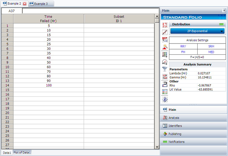
14 units were being reliability tested and the following life test data were obtained. Assuming that the data follow a 2-parameter exponential distribution, estimate the parameters and determine the correlation coefficient, [math]\displaystyle{ \rho \,\! }[/math], using rank regression on Y (RRY).

Life Test Data
Data point index	Time-to-failure
1	5
2	10
3	15
4	20
5	25
6	30
7	35
8	40
9	50
10	60
11	70
12	80
13	90
14	100

Solution

Construct the following table, as shown next.

[math]\displaystyle{ \overset{{}}{\mathop{\text{Table}\text{- Least Squares Analysis}}}\,\,\! }[/math] [math]\displaystyle{ \begin{matrix} N & t_{i} & F(t_{i}) & y_{i} & t_{i}^{2} & y_{i}^{2} & t_{i} y_{i} \\ \text{1} & \text{5} & \text{0}\text{.0483} & \text{-0}\text{.0495} & \text{25} & \text{0}\text{.0025} & \text{-0}\text{.2475} \\ \text{2} & \text{10} & \text{0}\text{.1170} & \text{-0}\text{.1244} & \text{100} & \text{0}\text{.0155} & \text{-1}\text{.2443} \\ \text{3} & \text{15} & \text{0}\text{.1865} & \text{-0}\text{.2064} & \text{225} & \text{0}\text{.0426} & \text{-3}\text{.0961} \\ \text{4} & \text{20} & \text{0}\text{.2561} & \text{-0}\text{.2958} & \text{400} & \text{0}\text{.0875} & \text{-5}\text{.9170} \\ \text{5} & \text{25} & \text{0}\text{.3258} & \text{-0}\text{.3942} & \text{625} & \text{0}\text{.1554} & \text{-9}\text{.8557} \\ \text{6} & \text{30} & \text{0}\text{.3954} & \text{-0}\text{.5032} & \text{900} & \text{0}\text{.2532} & \text{-15}\text{.0956} \\ \text{7} & \text{35} & \text{0}\text{.4651} & \text{-0}\text{.6257} & \text{1225} & \text{0}\text{.3915} & \text{-21}\text{.8986} \\ \text{8} & \text{40} & \text{0}\text{.5349} & \text{-0}\text{.7655} & \text{1600} & \text{0}\text{.5860} & \text{-30}\text{.6201} \\ \text{9} & \text{50} & \text{0}\text{.6046} & \text{-0}\text{.9279} & \text{2500} & \text{0}\text{.8609} & \text{-46}\text{.3929} \\ \text{10} & \text{60} & \text{0}\text{.6742} & \text{-1}\text{.1215} & \text{3600} & \text{1}\text{.2577} & \text{-67}\text{.2883} \\ \text{11} & \text{70} & \text{0}\text{.7439} & \text{-1}\text{.3622} & \text{4900} & \text{1}\text{.8456} & \text{-95}\text{.3531} \\ \text{12} & \text{80} & \text{0}\text{.8135} & \text{-1}\text{.6793} & \text{6400} & \text{2}\text{.8201} & \text{-134}\text{.3459} \\ \text{13} & \text{90} & \text{0}\text{.8830} & \text{-2}\text{.1456} & \text{8100} & \text{4}\text{.6035} & \text{-193}\text{.1023} \\ \text{14} & \text{100} & \text{0}\text{.9517} & \text{-3}\text{.0303} & \text{10000} & \text{9}\text{.1829} & \text{-303}\text{.0324} \\ \sum_{}^{} & \text{630} & {} & \text{-13}\text{.2315} & \text{40600} & \text{22}\text{.1148} & \text{-927}\text{.4899} \\ \end{matrix}\,\! }[/math]

The median rank values ( [math]\displaystyle{ F({{t}_{i}})\,\! }[/math] ) can be found in rank tables or they can be estimated using the Quick Statistical Reference in Weibull++. Given the values in the table above, calculate [math]\displaystyle{ \hat{a}\,\! }[/math] and [math]\displaystyle{ \hat{b}\,\! }[/math]:

[math]\displaystyle{ \begin{align} \hat{b}= & \frac{\underset{i=1}{\overset{14}{\mathop{\sum }}}\,{{t}_{i}}{{y}_{i}}-(\underset{i=1}{\overset{14}{\mathop{\sum }}}\,{{t}_{i}})(\underset{i=1}{\overset{14}{\mathop{\sum }}}\,{{y}_{i}})/14}{\underset{i=1}{\overset{14}{\mathop{\sum }}}\,t_{i}^{2}-{{(\underset{i=1}{\overset{14}{\mathop{\sum }}}\,{{t}_{i}})}^{2}}/14} \\ \\ \hat{b}= & \frac{-927.4899-(630)(-13.2315)/14}{40,600-{{(630)}^{2}}/14} \end{align}\,\! }[/math]

or:

[math]\displaystyle{ \hat{b}=-0.02711\,\! }[/math]

and:

[math]\displaystyle{ \hat{a}=\overline{y}-\hat{b}\overline{t}=\frac{\underset{i=1}{\overset{N}{\mathop{\sum }}}\,{{y}_{i}}}{N}-\hat{b}\frac{\underset{i=1}{\overset{N}{\mathop{\sum }}}\,{{t}_{i}}}{N}\,\! }[/math]

or:

[math]\displaystyle{ \hat{a}=\frac{-13.2315}{14}-(-0.02711)\frac{630}{14}=0.2748\,\! }[/math]

Therefore:

[math]\displaystyle{ \hat{\lambda }=-\hat{b}=-(-0.02711)=0.02711\text{ failures/hour}\,\! }[/math]

and:

[math]\displaystyle{ \hat{\gamma }=\frac{\hat{a}}{\hat{\lambda }}=\frac{0.2748}{0.02711}\,\! }[/math]

or:

[math]\displaystyle{ \hat{\gamma }=10.1365\text{ hours}\,\! }[/math]

Then:

[math]\displaystyle{ f(t)=(0.02711)\cdot {{e}^{-0.02711(T-10.136)}}\,\! }[/math]

The correlation coefficient can be estimated using equation for calculating the correlation coefficient:

[math]\displaystyle{ \hat{\rho }=-0.9679\,\! }[/math]

This example can be repeated using Weibull++, choosing 2-parameter exponential and rank regression on Y (RRY), as shown next.

The estimated parameters and the correlation coefficient using Weibull++ were found to be:

[math]\displaystyle{ \hat{\lambda }=0.0271\text{ fr/hr },\hat{\gamma }=10.1348\text{ hr },\hat{\rho }=-0.9679\,\! }[/math]

Please note that the user must deselect the Reset if location parameter > T1 on Exponential option on the Calculations page of the Application Setup window.

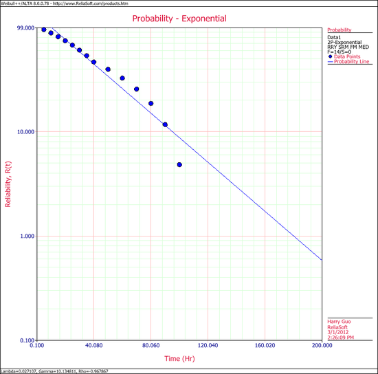
The probability plot can be obtained simply by clicking the Plot icon.