Template:Duane
Duane
Model History and Development
In 1962, J. T. Duane published a report in which he presented failure data of different systems during their development programs [8]. While analyzing the data, it was observed that the cumulative MTBF versus cumulative operating time followed a straight line when plotted on log-log paper (Figure oldpic71).
Based on that observation, Duane developed his model as follows. If
The equation of the line can be expressed as:
- Setting:
- yields:

Then equating
- or:
And, if you assume a constant failure intensity, then the cumulative failure intensity,
- or:
Also, the expected number of failures up to time
- where:
The corresponding
where
Similarly, using Eqn. (duanecnew), this procedure yields:
where

In 1962, J. T. Duane published a report in which he presented failure data of different systems during their development programs [8]. While analyzing the data, it was observed that the cumulative MTBF versus cumulative operating time followed a straight line when plotted on log-log paper, as shown next.
Based on that observation, Duane developed his model as follows. If
The equation of the line can be expressed as:
Setting:
yields:
Then equating
or:
And, if you assume a constant failure intensity, then the cumulative failure intensity,
or:
Also, the expected number of failures up to time
where:
The corresponding
where
The cumulative MTBF,
Similarly, using the equation for the expected number of failures up to time
where
As shown in these derivations, the instantaneous failure intensity improvement line is obtained by shifting the cumulative failure intensity line down, parallel to itself, by a distance of
Parameter Estimation
The Duane model is a two parameter model. Therefore, to use this model as a basis for predicting the reliability growth that could be expected in an equipment development program, procedures must be defined for estimating these parameters as a function of equipment characteristics. Note that, while these parameters can be estimated for a given data set using curve-fitting methods, there exists no underlying theory for the Duane model that could provide a basis for a priori estimation.
One of the parameters of the Duane model is

Graphical Method
The Duane model for the cumulative failure intensity is:
This equation may be linearized by taking the natural log of both sides:
Consequently, plotting
Similarly, the corresponding MTBF of the cumulative failure intensity can also be linearized by taking the natural log of both sides:
Plotting
Two ways of determining these curves are as follows:
1. Predict the
| Equipment | Slope( | |
|---|---|---|
| Computer system | Actual | 0.24 |
| Easy to find failures were eliminated | 0.26 | |
| All known failure causes were eliminated | 0.36 | |
| Mainframe computer | 0.50 | |
| Aerospace electronics | All malfunctions | 0.57 |
| Relevant failures only | 0.65 | |
| Attack radar | 0.60 | |
| Rocket engine | 0.46 | |
| Afterburning turbojet | 0.35 | |
| Complex hydromechanical system | 0.60 | |
| Aircraft generator | 0.38 | |
| Modern dry turbojet | 0.48 |
2. During the design, development and test phase and at specific milestones, the
Graphical Method Example
A complex system's reliability growth is being monitored and the data set is given in the table below.
| Point Number | Cumulative Test Time(hours) | Cumulative Failures | Cumulative MTBF(hours) | Instantaneous MTBF(hours) |
|---|---|---|---|---|
| 1 | 200 | 2 | 100.0 | 100 |
| 2 | 400 | 3 | 133.0 | 200 |
| 3 | 600 | 4 | 150.0 | 200 |
| 4 | 3,000 | 11 | 273.0 | 342.8 |
Do the following:
- Plot the cumulative MTBF growth curve.
- Write the equation of this growth curve.
- Write the equation of the instantaneous MTBF growth model.
- Plot the instantaneous MTBF growth curve.
Solution
- Given the data in the second and third columns of the above table, the cumulative MTBF,
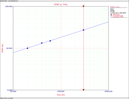
Cumulative MTBF plot 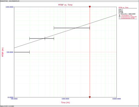
Instantaneous MTBF plot By changing the x-axis scaling, you are able to extend the line to
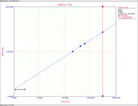
Cumulative MTBF plot for Another way of determining
Then substitute this
Using the cumulative MTBF plot for the example, at
- Substituting the second set of values,
- Now the equation for the cumulative MTBF growth curve is:
- Using the following equation for the instantaneous MTBF, or
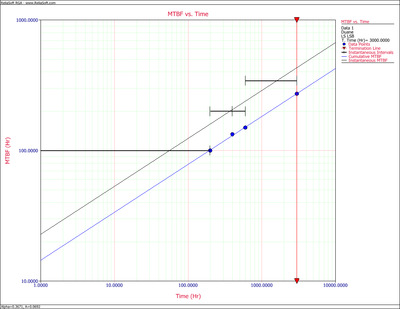
Cumulative and Instantaneous MTBF vs. Time plot


Least Squares (Linear Regression)
The parameters can also be estimated using a mathematical approach. To do this, linearize the MTBF of the cumulative failure intensity by taking the natural log of both sides, and then apply least squares analysis. For example:
For simplicity in the calculations, let:
Therefore, the equation becomes:
Assume that a set of data pairs
where
Differentiating
and:
Set those two equations equal to zero:
and:
Solve the equations simultaneously:
and:
Now substituting back
where:
Example 1
Using the same data set from the graphical approach example, estimate the parameters of the MTBF model using least squares.
Solution
From the data table:
Obtain the value of
Obtain the value
Therefore, the cumulative MTBF becomes:
The equation for the instantaneous MTBF growth curve is:
Example 2
For the data given in columns 1 and 2 of the following table, estimate the Duane parameters using least squares.
| (1)Failure Number | (2)Failure Time(hours) | (3) |
(4) |
(5) |
(6) |
(7) |
|---|---|---|---|---|---|---|
| 1 | 9.2 | 2.219 | 4.925 | 9.200 | 2.219 | 4.925 |
| 2 | 25 | 3.219 | 10.361 | 12.500 | 2.526 | 8.130 |
| 3 | 61.5 | 4.119 | 16.966 | 20.500 | 3.020 | 12.441 |
| 4 | 260 | 5.561 | 30.921 | 65.000 | 4.174 | 23.212 |
| 5 | 300 | 5.704 | 32.533 | 60.000 | 4.094 | 23.353 |
| 6 | 710 | 6.565 | 43.103 | 118.333 | 4.774 | 31.339 |
| 7 | 916 | 6.820 | 46.513 | 130.857 | 4.874 | 33.241 |
| 8 | 1010 | 6.918 | 47.855 | 126.250 | 4.838 | 33.470 |
| 9 | 1220 | 7.107 | 50.504 | 135.556 | 4.909 | 34.889 |
| 10 | 2530 | 7.836 | 61.402 | 253.000 | 5.533 | 43.359 |
| 11 | 3350 | 8.117 | 65.881 | 304.545 | 5.719 | 46.418 |
| 12 | 4200 | 8.343 | 69.603 | 350.000 | 5.858 | 48.872 |
| 13 | 4410 | 8.392 | 70.419 | 339.231 | 5.827 | 48.895 |
| 14 | 4990 | 8.515 | 72.508 | 356.429 | 5.876 | 50.036 |
| 15 | 5570 | 8.625 | 74.393 | 371.333 | 5.917 | 51.036 |
| 16 | 8310 | 9.025 | 81.455 | 519.375 | 6.253 | 56.431 |
| 17 | 8530 | 9.051 | 81.927 | 501.765 | 6.218 | 56.282 |
| 18 | 9200 | 9.127 | 83.301 | 511.111 | 6.237 | 56.921 |
| 19 | 10500 | 9.259 | 85.731 | 552.632 | 6.315 | 58.469 |
| 20 | 12100 | 9.401 | 88.378 | 605.000 | 6.405 | 60.215 |
| 21 | 13400 | 9.503 | 90.307 | 638.095 | 6.458 | 61.375 |
| 22 | 14600 | 9.589 | 91.945 | 663.636 | 6.498 | 62.305 |
| 23 | 22000 | 9.999 | 99.976 | 956.522 | 6.863 | 68.625 |
| Sum = | 173.013 | 1400.908 | 7600.870 | 121.406 | 974.242 |
Solution
To estimate the parameters using least squares, the values in columns 3, 4, 5, 6 and 7 are calculated. The cumulative MTBF,
The estimator of
Therefore, the cumulative MTBF becomes:
Using the equation for the instantaneous MTBF growth curve,

Example 3
For the data given in the following table, estimate the Duane parameters using least squares.
| Run Number | Failed Unit | Test Time 1 | Test Time 2 | Cumulative Time |
|---|---|---|---|---|
| 1 | 1 | 0.2 | 2.0 | 2.2 |
| 2 | 2 | 1.7 | 2.9 | 4.6 |
| 3 | 2 | 4.5 | 5.2 | 9.7 |
| 4 | 2 | 5.8 | 9.1 | 14.9 |
| 5 | 2 | 17.3 | 9.2 | 26.5 |
| 6 | 2 | 29.3 | 24.1 | 53.4 |
| 7 | 1 | 36.5 | 61.1 | 97.6 |
| 8 | 2 | 46.3 | 69.6 | 115.9 |
| 9 | 1 | 63.6 | 78.1 | 141.7 |
| 10 | 2 | 64.4 | 85.4 | 149.8 |
| 11 | 1 | 74.3 | 93.6 | 167.9 |
| 12 | 1 | 106.6 | 103 | 209.6 |
| 13 | 2 | 195.2 | 117 | 312.2 |
| 14 | 2 | 235.1 | 134.3 | 369.4 |
| 15 | 1 | 248.7 | 150.2 | 398.9 |
| 16 | 2 | 256.8 | 164.6 | 421.4 |
| 17 | 2 | 261.1 | 174.3 | 435.4 |
| 18 | 2 | 299.4 | 193.2 | 492.6 |
| 19 | 1 | 305.3 | 234.2 | 539.5 |
| 20 | 1 | 326.9 | 257.3 | 584.2 |
| 21 | 1 | 339.2 | 290.2 | 629.4 |
| 22 | 1 | 366.1 | 293.1 | 659.2 |
| 23 | 2 | 466.4 | 316.4 | 782.8 |
| 24 | 1 | 504 | 373.2 | 877.2 |
| 25 | 1 | 510 | 375.1 | 885.1 |
| 26 | 2 | 543.2 | 386.1 | 929.3 |
| 27 | 2 | 635.4 | 453.3 | 1088.7 |
| 28 | 1 | 641.2 | 485.8 | 1127 |
| 29 | 2 | 755.8 | 573.6 | 1329.4 |
Solution
The solution to this example follows the same procedure as the previous example. Therefore, from the table shown above:
For least squares, the value of
The value of the estimator
Therefore, the cumulative MTBF is:
Using the equation for the instantaneous MTBF growth,
Maximum Likelihood Estimators
L. H. Crow [17] noted that the Duane model could be stochastically represented as a Weibull process, allowing for statistical procedures to be used in the application of this model in reliability growth. This statistical extension became what is known as the Crow-AMSAA (NHPP) model. The Crow-AMSAA model, which is described in the Crow-AMSAA (NHPP) chapter, provides a complete Maximum Likelihood Estimation (MLE) solution to the Duane model.
Confidence Bounds
Least squares confidence bounds can be computed for both the model parameters and metrics of interest for the Duane model.
Parameter Bounds
Apply least squares analysis on the Duane model:
The unbiased estimator of
where:
Thus, the confidence bounds on
where
Other Bounds
Confidence bounds also can be obtained on the cumulative MTBF and the cumulative failure intensity:
When
and
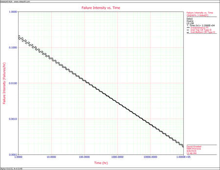
therefore, the confidence bounds on the instantaneous failure intensity are:
Duane Confidence Bounds Example
Using the values of
Calculate the 90% confidence bounds for the following:
- The parameters
- The cumulative and instantaneous failure intensity.
- The cumulative and instantaneous MTBF.
Solution
- Use the values of
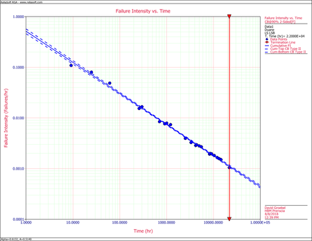
- The cumulative failure intensity is:
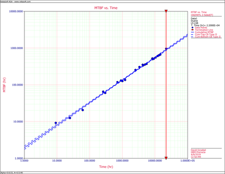
- The cumulative MTBF is:
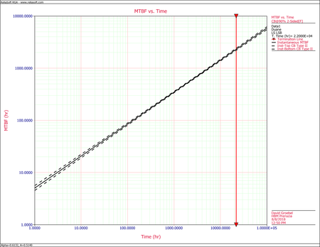
The next figure displays the instantaneous MTBF. Both are plotted with confidence bounds.


More Examples
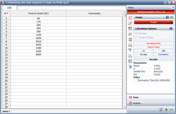
Estimating the Time Required to Meet an MTBF Goal
A prototype of a system was tested with design changes incorporated during the test. A total of 12 failures occurred. The data set is given in the following table.
| Failure Number | Cumulative Test Time(hours) |
|---|---|
| 1 | 80 |
| 2 | 175 |
| 3 | 265 |
| 4 | 400 |
| 5 | 590 |
| 6 | 1100 |
| 7 | 1650 |
| 8 | 2010 |
| 9 | 2400 |
| 10 | 3380 |
| 11 | 5100 |
| 12 | 6400 |
Do the following:
- Estimate the Duane parameters.
- Plot the cumulative and instantaneous MTBF curves.
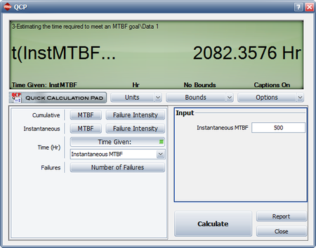
- How many cumulative test and development hours are required to meet an instantaneous MTBF goal of 500 hours?
- How many cumulative test and development hours are required to meet a cumulative MTBF goal of 500 hours?
Solution
- The next figure shows the data entered into RGA along with the estimated Duane parameters.
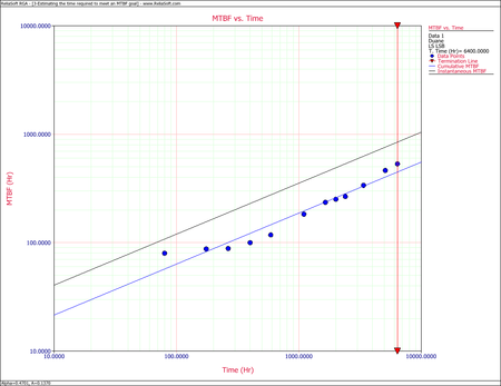
- The following figure shows the cumulative and instantaneous MTBF curves.
- The next figure shows the cumulative test and development hours needed for an instantaneous MTBF goal of 500 hours.
- The figure below shows the cumulative test and development hours needed for a cumulative MTBF goal of 500 hours.


Multiple Systems - Known Operating Times Example
Two identical systems were tested. Any design changes made to improve the reliability of these systems were incorporated into both systems when any system failed. A total of 29 failures occurred. The data set is given in the table below.
Do the following:
- Estimate the Duane parameters.
- Assume both units are tested for an additional 100 hours each. How many failures do you expect in that period?
- If testing/development were halted at this point, what would the reliability equation for this system be?
| Failure Number | Failed Unit | Test Time Unit 1(hours) | Test Time Unit 2 (hours) |
|---|---|---|---|
| 1 | 1 | 0.2 | 2.0 |
| 2 | 2 | 1.7 | 2.9 |
| 3 | 2 | 4.5 | 5.2 |
| 4 | 2 | 5.8 | 9.1 |
| 5 | 2 | 17.3 | 9.2 |
| 6 | 2 | 29.3 | 24.1 |
| 7 | 1 | 36.5 | 61.1 |
| 8 | 2 | 46.3 | 69.6 |
| 9 | 1 | 63.6 | 78.1 |
| 10 | 2 | 64.4 | 85.4 |
| 11 | 1 | 74.3 | 93.6 |
| 12 | 1 | 106.6 | 103 |
| 13 | 2 | 195.2 | 117 |
| 14 | 2 | 235.1 | 134.3 |
| 15 | 1 | 248.7 | 150.2 |
| 16 | 2 | 256.8 | 164.6 |
| 17 | 2 | 261.1 | 174.3 |
| 18 | 2 | 299.4 | 193.2 |
| 19 | 1 | 305.3 | 234.2 |
| 20 | 1 | 326.9 | 257.3 |
| 21 | 1 | 339.2 | 290.2 |
| 22 | 1 | 366.1 | 293.1 |
| 23 | 2 | 466.4 | 316.4 |
| 24 | 1 | 504 | 373.2 |
| 25 | 1 | 510 | 375.1 |
| 26 | 2 | 543.2 | 386.1 |
| 27 | 2 | 635.4 | 453.3 |
| 28 | 1 | 641.2 | 485.8 |
| 29 | 2 | 755.8 | 573.6 |
Solution
- The figure below shows the data entered into RGA along with the estimated Duane parameters.
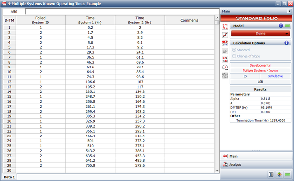
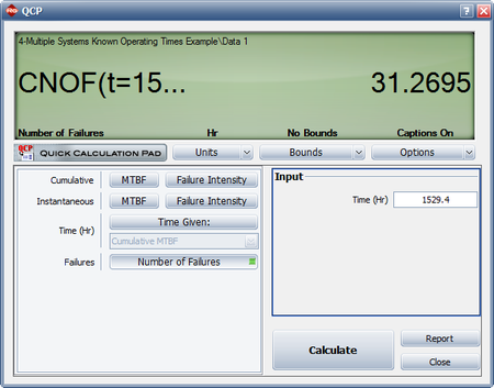
- The current accumulated test time for both units is 1329.4 hours. If the process were to continue for an additional combined time of 200 hours, the expected cumulative number of failures at
- If testing/development were halted at this point, the system failure intensity would be equal to the instantaneous failure intensity at that time, or
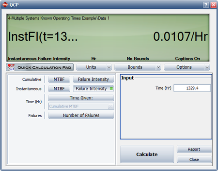
An exponential distribution can be assumed since the value of the failure intensity at that instant in time is known. Therefore:
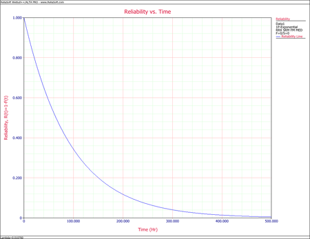
Weibull++ can be utilized to provide a Reliability vs. Time plot which is shown below.


Using the Duane Model for Success/Failure Data
Given the sequential success/failure data in the table below, do the following:
- Estimate the Duane parameters.
- What is the instantaneous Reliability at the end of the test?
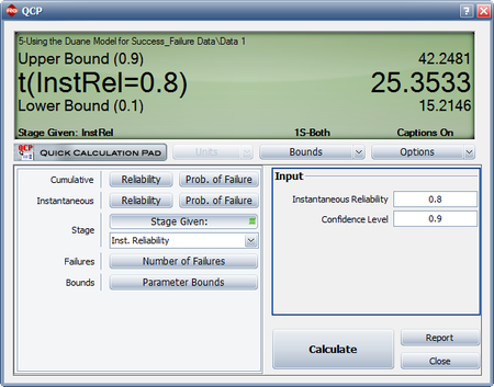
- How many additional test runs with a one-sided 90% confidence level are required to meet an instantaneous Reliability goal of 80%?
| Run Number | Result |
|---|---|
| 1 | F |
| 2 | F |
| 3 | S |
| 4 | S |
| 5 | S |
| 6 | F |
| 7 | S |
| 8 | F |
| 9 | F |
| 10 | S |
| 11 | S |
| 12 | S |
| 13 | F |
| 14 | S |
| 15 | S |
| 16 | S |
| 17 | S |
| 18 | S |
| 19 | S |
| 20 | S |
Solution
- The following figure shows the data set entered into RGA along with the estimated Duane parameters.
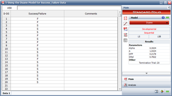
- The Reliability at the end of the test is equal to 78.22%. Note that this is the DRel that is shown in the control panel in the above figure.
- The figure below shows the number of test runs with both one-sided confidence bounds at 90% confidence level to achieve an instantaneous Reliability of 80%. Therefore, the number of additional test runs required with a 90% confidence level is equal to


In 1962, J. T. Duane published a report in which he presented failure data of different systems during their development programs [8]. While analyzing the data, it was observed that the cumulative MTBF versus cumulative operating time followed a straight line when plotted on log-log paper, as shown next.
Based on that observation, Duane developed his model as follows. If
The equation of the line can be expressed as:
Setting:
yields:
Then equating
or:
And, if you assume a constant failure intensity, then the cumulative failure intensity,
or:
Also, the expected number of failures up to time
where:
The corresponding
where
The cumulative MTBF,
Similarly, using the equation for the expected number of failures up to time
where
As shown in these derivations, the instantaneous failure intensity improvement line is obtained by shifting the cumulative failure intensity line down, parallel to itself, by a distance of
Parameter Estimation
The Duane model is a two parameter model. Therefore, to use this model as a basis for predicting the reliability growth that could be expected in an equipment development program, procedures must be defined for estimating these parameters as a function of equipment characteristics. Note that, while these parameters can be estimated for a given data set using curve-fitting methods, there exists no underlying theory for the Duane model that could provide a basis for a priori estimation.
One of the parameters of the Duane model is
Graphical Method
The Duane model for the cumulative failure intensity is:
This equation may be linearized by taking the natural log of both sides:
Consequently, plotting
Similarly, the corresponding MTBF of the cumulative failure intensity can also be linearized by taking the natural log of both sides:
Plotting
Two ways of determining these curves are as follows:
1. Predict the
| Equipment | Slope( | |
|---|---|---|
| Computer system | Actual | 0.24 |
| Easy to find failures were eliminated | 0.26 | |
| All known failure causes were eliminated | 0.36 | |
| Mainframe computer | 0.50 | |
| Aerospace electronics | All malfunctions | 0.57 |
| Relevant failures only | 0.65 | |
| Attack radar | 0.60 | |
| Rocket engine | 0.46 | |
| Afterburning turbojet | 0.35 | |
| Complex hydromechanical system | 0.60 | |
| Aircraft generator | 0.38 | |
| Modern dry turbojet | 0.48 |
2. During the design, development and test phase and at specific milestones, the
Graphical Method Example
A complex system's reliability growth is being monitored and the data set is given in the table below.
| Point Number | Cumulative Test Time(hours) | Cumulative Failures | Cumulative MTBF(hours) | Instantaneous MTBF(hours) |
|---|---|---|---|---|
| 1 | 200 | 2 | 100.0 | 100 |
| 2 | 400 | 3 | 133.0 | 200 |
| 3 | 600 | 4 | 150.0 | 200 |
| 4 | 3,000 | 11 | 273.0 | 342.8 |
Do the following:
- Plot the cumulative MTBF growth curve.
- Write the equation of this growth curve.
- Write the equation of the instantaneous MTBF growth model.
- Plot the instantaneous MTBF growth curve.
Solution
- Given the data in the second and third columns of the above table, the cumulative MTBF,
Cumulative MTBF plot Instantaneous MTBF plot By changing the x-axis scaling, you are able to extend the line to
Cumulative MTBF plot for Another way of determining
Then substitute this
Using the cumulative MTBF plot for the example, at
- Substituting the second set of values,
- Now the equation for the cumulative MTBF growth curve is:
- Using the following equation for the instantaneous MTBF, or
Cumulative and Instantaneous MTBF vs. Time plot
Least Squares (Linear Regression)
The parameters can also be estimated using a mathematical approach. To do this, linearize the MTBF of the cumulative failure intensity by taking the natural log of both sides, and then apply least squares analysis. For example:
For simplicity in the calculations, let:
Therefore, the equation becomes:
Assume that a set of data pairs
where
Differentiating
and:
Set those two equations equal to zero:
and:
Solve the equations simultaneously:
and:
Now substituting back
where:
Example 1
Using the same data set from the graphical approach example, estimate the parameters of the MTBF model using least squares.
Solution
From the data table:
Obtain the value of
Obtain the value
Therefore, the cumulative MTBF becomes:
The equation for the instantaneous MTBF growth curve is:
Example 2
For the data given in columns 1 and 2 of the following table, estimate the Duane parameters using least squares.
| (1)Failure Number | (2)Failure Time(hours) | (3) |
(4) |
(5) |
(6) |
(7) |
|---|---|---|---|---|---|---|
| 1 | 9.2 | 2.219 | 4.925 | 9.200 | 2.219 | 4.925 |
| 2 | 25 | 3.219 | 10.361 | 12.500 | 2.526 | 8.130 |
| 3 | 61.5 | 4.119 | 16.966 | 20.500 | 3.020 | 12.441 |
| 4 | 260 | 5.561 | 30.921 | 65.000 | 4.174 | 23.212 |
| 5 | 300 | 5.704 | 32.533 | 60.000 | 4.094 | 23.353 |
| 6 | 710 | 6.565 | 43.103 | 118.333 | 4.774 | 31.339 |
| 7 | 916 | 6.820 | 46.513 | 130.857 | 4.874 | 33.241 |
| 8 | 1010 | 6.918 | 47.855 | 126.250 | 4.838 | 33.470 |
| 9 | 1220 | 7.107 | 50.504 | 135.556 | 4.909 | 34.889 |
| 10 | 2530 | 7.836 | 61.402 | 253.000 | 5.533 | 43.359 |
| 11 | 3350 | 8.117 | 65.881 | 304.545 | 5.719 | 46.418 |
| 12 | 4200 | 8.343 | 69.603 | 350.000 | 5.858 | 48.872 |
| 13 | 4410 | 8.392 | 70.419 | 339.231 | 5.827 | 48.895 |
| 14 | 4990 | 8.515 | 72.508 | 356.429 | 5.876 | 50.036 |
| 15 | 5570 | 8.625 | 74.393 | 371.333 | 5.917 | 51.036 |
| 16 | 8310 | 9.025 | 81.455 | 519.375 | 6.253 | 56.431 |
| 17 | 8530 | 9.051 | 81.927 | 501.765 | 6.218 | 56.282 |
| 18 | 9200 | 9.127 | 83.301 | 511.111 | 6.237 | 56.921 |
| 19 | 10500 | 9.259 | 85.731 | 552.632 | 6.315 | 58.469 |
| 20 | 12100 | 9.401 | 88.378 | 605.000 | 6.405 | 60.215 |
| 21 | 13400 | 9.503 | 90.307 | 638.095 | 6.458 | 61.375 |
| 22 | 14600 | 9.589 | 91.945 | 663.636 | 6.498 | 62.305 |
| 23 | 22000 | 9.999 | 99.976 | 956.522 | 6.863 | 68.625 |
| Sum = | 173.013 | 1400.908 | 7600.870 | 121.406 | 974.242 |
Solution
To estimate the parameters using least squares, the values in columns 3, 4, 5, 6 and 7 are calculated. The cumulative MTBF,
The estimator of
Therefore, the cumulative MTBF becomes:
Using the equation for the instantaneous MTBF growth curve,
Example 3
For the data given in the following table, estimate the Duane parameters using least squares.
| Run Number | Failed Unit | Test Time 1 | Test Time 2 | Cumulative Time |
|---|---|---|---|---|
| 1 | 1 | 0.2 | 2.0 | 2.2 |
| 2 | 2 | 1.7 | 2.9 | 4.6 |
| 3 | 2 | 4.5 | 5.2 | 9.7 |
| 4 | 2 | 5.8 | 9.1 | 14.9 |
| 5 | 2 | 17.3 | 9.2 | 26.5 |
| 6 | 2 | 29.3 | 24.1 | 53.4 |
| 7 | 1 | 36.5 | 61.1 | 97.6 |
| 8 | 2 | 46.3 | 69.6 | 115.9 |
| 9 | 1 | 63.6 | 78.1 | 141.7 |
| 10 | 2 | 64.4 | 85.4 | 149.8 |
| 11 | 1 | 74.3 | 93.6 | 167.9 |
| 12 | 1 | 106.6 | 103 | 209.6 |
| 13 | 2 | 195.2 | 117 | 312.2 |
| 14 | 2 | 235.1 | 134.3 | 369.4 |
| 15 | 1 | 248.7 | 150.2 | 398.9 |
| 16 | 2 | 256.8 | 164.6 | 421.4 |
| 17 | 2 | 261.1 | 174.3 | 435.4 |
| 18 | 2 | 299.4 | 193.2 | 492.6 |
| 19 | 1 | 305.3 | 234.2 | 539.5 |
| 20 | 1 | 326.9 | 257.3 | 584.2 |
| 21 | 1 | 339.2 | 290.2 | 629.4 |
| 22 | 1 | 366.1 | 293.1 | 659.2 |
| 23 | 2 | 466.4 | 316.4 | 782.8 |
| 24 | 1 | 504 | 373.2 | 877.2 |
| 25 | 1 | 510 | 375.1 | 885.1 |
| 26 | 2 | 543.2 | 386.1 | 929.3 |
| 27 | 2 | 635.4 | 453.3 | 1088.7 |
| 28 | 1 | 641.2 | 485.8 | 1127 |
| 29 | 2 | 755.8 | 573.6 | 1329.4 |
Solution
The solution to this example follows the same procedure as the previous example. Therefore, from the table shown above:
For least squares, the value of
The value of the estimator
Therefore, the cumulative MTBF is:
Using the equation for the instantaneous MTBF growth,
Maximum Likelihood Estimators
L. H. Crow [17] noted that the Duane model could be stochastically represented as a Weibull process, allowing for statistical procedures to be used in the application of this model in reliability growth. This statistical extension became what is known as the Crow-AMSAA (NHPP) model. The Crow-AMSAA model, which is described in the Crow-AMSAA (NHPP) chapter, provides a complete Maximum Likelihood Estimation (MLE) solution to the Duane model.
Confidence Bounds
Least squares confidence bounds can be computed for both the model parameters and metrics of interest for the Duane model.
Parameter Bounds
Apply least squares analysis on the Duane model:
The unbiased estimator of
where:
Thus, the confidence bounds on
where
Other Bounds
Confidence bounds also can be obtained on the cumulative MTBF and the cumulative failure intensity:
When
and
therefore, the confidence bounds on the instantaneous failure intensity are:
Duane Confidence Bounds Example
Using the values of
Calculate the 90% confidence bounds for the following:
- The parameters
- The cumulative and instantaneous failure intensity.
- The cumulative and instantaneous MTBF.
Solution
- Use the values of
- The cumulative failure intensity is:
- The cumulative MTBF is:
The next figure displays the instantaneous MTBF. Both are plotted with confidence bounds.
More Examples
Estimating the Time Required to Meet an MTBF Goal
A prototype of a system was tested with design changes incorporated during the test. A total of 12 failures occurred. The data set is given in the following table.
| Failure Number | Cumulative Test Time(hours) |
|---|---|
| 1 | 80 |
| 2 | 175 |
| 3 | 265 |
| 4 | 400 |
| 5 | 590 |
| 6 | 1100 |
| 7 | 1650 |
| 8 | 2010 |
| 9 | 2400 |
| 10 | 3380 |
| 11 | 5100 |
| 12 | 6400 |
Do the following:
- Estimate the Duane parameters.
- Plot the cumulative and instantaneous MTBF curves.
- How many cumulative test and development hours are required to meet an instantaneous MTBF goal of 500 hours?
- How many cumulative test and development hours are required to meet a cumulative MTBF goal of 500 hours?
Solution
- The next figure shows the data entered into RGA along with the estimated Duane parameters.
- The following figure shows the cumulative and instantaneous MTBF curves.
- The next figure shows the cumulative test and development hours needed for an instantaneous MTBF goal of 500 hours.
- The figure below shows the cumulative test and development hours needed for a cumulative MTBF goal of 500 hours.
Multiple Systems - Known Operating Times Example
Two identical systems were tested. Any design changes made to improve the reliability of these systems were incorporated into both systems when any system failed. A total of 29 failures occurred. The data set is given in the table below.
Do the following:
- Estimate the Duane parameters.
- Assume both units are tested for an additional 100 hours each. How many failures do you expect in that period?
- If testing/development were halted at this point, what would the reliability equation for this system be?
| Failure Number | Failed Unit | Test Time Unit 1(hours) | Test Time Unit 2 (hours) |
|---|---|---|---|
| 1 | 1 | 0.2 | 2.0 |
| 2 | 2 | 1.7 | 2.9 |
| 3 | 2 | 4.5 | 5.2 |
| 4 | 2 | 5.8 | 9.1 |
| 5 | 2 | 17.3 | 9.2 |
| 6 | 2 | 29.3 | 24.1 |
| 7 | 1 | 36.5 | 61.1 |
| 8 | 2 | 46.3 | 69.6 |
| 9 | 1 | 63.6 | 78.1 |
| 10 | 2 | 64.4 | 85.4 |
| 11 | 1 | 74.3 | 93.6 |
| 12 | 1 | 106.6 | 103 |
| 13 | 2 | 195.2 | 117 |
| 14 | 2 | 235.1 | 134.3 |
| 15 | 1 | 248.7 | 150.2 |
| 16 | 2 | 256.8 | 164.6 |
| 17 | 2 | 261.1 | 174.3 |
| 18 | 2 | 299.4 | 193.2 |
| 19 | 1 | 305.3 | 234.2 |
| 20 | 1 | 326.9 | 257.3 |
| 21 | 1 | 339.2 | 290.2 |
| 22 | 1 | 366.1 | 293.1 |
| 23 | 2 | 466.4 | 316.4 |
| 24 | 1 | 504 | 373.2 |
| 25 | 1 | 510 | 375.1 |
| 26 | 2 | 543.2 | 386.1 |
| 27 | 2 | 635.4 | 453.3 |
| 28 | 1 | 641.2 | 485.8 |
| 29 | 2 | 755.8 | 573.6 |
Solution
- The figure below shows the data entered into RGA along with the estimated Duane parameters.
- The current accumulated test time for both units is 1329.4 hours. If the process were to continue for an additional combined time of 200 hours, the expected cumulative number of failures at
- If testing/development were halted at this point, the system failure intensity would be equal to the instantaneous failure intensity at that time, or
An exponential distribution can be assumed since the value of the failure intensity at that instant in time is known. Therefore:
Weibull++ can be utilized to provide a Reliability vs. Time plot which is shown below.
Using the Duane Model for Success/Failure Data
Given the sequential success/failure data in the table below, do the following:
- Estimate the Duane parameters.
- What is the instantaneous Reliability at the end of the test?
- How many additional test runs with a one-sided 90% confidence level are required to meet an instantaneous Reliability goal of 80%?
| Run Number | Result |
|---|---|
| 1 | F |
| 2 | F |
| 3 | S |
| 4 | S |
| 5 | S |
| 6 | F |
| 7 | S |
| 8 | F |
| 9 | F |
| 10 | S |
| 11 | S |
| 12 | S |
| 13 | F |
| 14 | S |
| 15 | S |
| 16 | S |
| 17 | S |
| 18 | S |
| 19 | S |
| 20 | S |
Solution
- The following figure shows the data set entered into RGA along with the estimated Duane parameters.
- The Reliability at the end of the test is equal to 78.22%. Note that this is the DRel that is shown in the control panel in the above figure.
- The figure below shows the number of test runs with both one-sided confidence bounds at 90% confidence level to achieve an instantaneous Reliability of 80%. Therefore, the number of additional test runs required with a 90% confidence level is equal to
General Examples
Example 6
A prototype of a system was tested with design changes incorporated during the test. A total of 12 failures occurred. The data set is given in Table 4.5.
- Estimate the Duane parameters.
- Plot the cumulative and instantaneous MTBF curves.
- How many cumulative test and development hours are required to meet an instantaneous MTBF goal #of 500 hours?
- How many cumulative test and development hours are required to meet a cumulative MTBF goal of 500 hours?
| Failure Number | Cumulative Test Time(hr) |
|---|---|
| 1 | 80 |
| 2 | 175 |
| 3 | 265 |
| 4 | 400 |
| 5 | 590 |
| 6 | 1100 |
| 7 | 1650 |
| 8 | 2010 |
| 9 | 2400 |
| 10 | 3380 |
| 11 | 5100 |
| 12 | 6400 |
Solution to Example 6
- Figure figuaneex11 shows the data entered into RGA along with the estimated Duane parameters.
- Figure figuaneex12 shows the cumulative and instantaneous MTBF curves.
- Figure figuaneex14 shows the cumulative test and development hours needed for an instantaneous MTBF goal of 500 hours.
- Figure figuaneex15 shows the cumulative test and development hours needed for a cumulative MTBF goal of 500 hours.
Example 7
Two identical systems were tested. Any design changes made to improve the reliability of these systems were incorporated into both systems when any system failed. A total of 29 failures occurred. The data set is given in Table 4.6. Do the following:
- Estimate the Duane parameters.
- Assume both units are tested for an additional 100 hrs each. How many failures do you expect in that period?
- If testing/development were halted at this point, what would the reliability equation for this system be
| Failure Number | Failed Unit | Test Time Unit 1(hr) | Test Time Unit 2 (hr) |
|---|---|---|---|
| 1 | 1 | 0.2 | 2.0 |
| 2 | 2 | 1.7 | 2.9 |
| 3 | 2 | 4.5 | 5.2 |
| 4 | 2 | 5.8 | 9.1 |
| 5 | 2 | 17.3 | 9.2 |
| 6 | 2 | 29.3 | 24.1 |
| 7 | 1 | 36.5 | 61.1 |
| 8 | 2 | 46.3 | 69.6 |
| 9 | 1 | 63.6 | 78.1 |
| 10 | 2 | 64.4 | 85.4 |
| 11 | 1 | 74.3 | 93.6 |
| 12 | 1 | 106.6 | 103 |
| 13 | 2 | 195.2 | 117 |
| 14 | 2 | 235.1 | 134.3 |
| 15 | 1 | 248.7 | 150.2 |
| 16 | 2 | 256.8 | 164.6 |
| 17 | 2 | 261.1 | 174.3 |
| 18 | 2 | 299.4 | 193.2 |
| 19 | 1 | 305.3 | 234.2 |
| 20 | 1 | 326.9 | 257.3 |
| 21 | 1 | 339.2 | 290.2 |
| 22 | 1 | 366.1 | 293.1 |
| 23 | 2 | 466.4 | 316.4 |
| 24 | 1 | 504 | 373.2 |
| 25 | 1 | 510 | 375.1 |
| 26 | 2 | 543.2 | 386.1 |
| 27 | 2 | 635.4 | 453.3 |
| 28 | 1 | 641.2 | 485.8 |
| 29 | 2 | 755.8 | 573.6 |
Solution to Example 7
- 1) Figure figuaneex21 shows the data entered into RGA along with the estimated Duane parameters.
- 2) The current accumulated test time for both units is 1329.4 hr. If the process were to continue for an additional combined time of 200 hr, the expected cumulative number of failures at
- 3) If testing/development were halted at this point, the system failure intensity would be equal to the instantaneous failure intensity at that time, or
Weibull++ can be utilized (from within RGA) to provide a Reliability vs. Time plot. This is shown in Figure figuaneex24.
Example 8
Given the sequential success/failure data in the Table 4.7, do the following:
- 1) Estimate the Duane parameters.
- 2) What is the instantaneous MTBF at the end of the test?
- 3) How many additional test runs with a one-sided 90% confidence level are required to meet an instantaneous MTBF goal of 5 hours?
| Run Number | Result |
|---|---|
| 1 | F |
| 2 | F |
| 3 | S |
| 4 | S |
| 5 | S |
| 6 | F |
| 7 | S |
| 8 | F |
| 9 | F |
| 10 | S |
| 11 | S |
| 12 | S |
| 13 | F |
| 14 | S |
| 15 | S |
| 16 | S |
| 17 | S |
| 18 | S |
| 19 | S |
| 20 | S |
Solution to Example 8
- 1) Figure figuaneex31 shows the data set entered into RGA along with the estimated Duane parameters.
- 2) The MTBF at the end of the test is equal to 4.5904 hours. Note that this is the DMTBF that is shown in the Control Panel in Figure figuaneex31.
- 3) Figure figuaneex34 shows the number of test runs with both one-sided confidence bounds at 90% confidence level to achieve an instantaneous MTBF of 5 hours. Therefore, the number of additional test runs required with a 90% confidence level is equal to