Template:Weibull++ Examples and Case Studies

Confidence Bound Example

Likelihood Ratio Bounds on Parameters

Likelihood Ratio Bounds on Parameters

Five units were put on a reliability test and experienced failures at 10, 20, 30, 40 and 50 hours. Assuming a Weibull distribution, the MLE parameter estimates are calculated to be [math]\displaystyle{ \widehat{\beta }=2.2938\,\! }[/math] and [math]\displaystyle{ \widehat{\eta }=33.9428.\,\! }[/math] Calculate the 90% two-sided confidence bounds on these parameters using the likelihood ratio method.

Solution

The first step is to calculate the likelihood function for the parameter estimates:

[math]\displaystyle{ \begin{align} L(\widehat{\beta },\widehat{\eta })= & \underset{i=1}{\overset{N}{\mathop \prod }}\,f({{x}_{i}};\widehat{\beta },\widehat{\eta })=\underset{i=1}{\overset{5}{\mathop \prod }}\,\frac{\widehat{\beta }}{\widehat{\eta }}\cdot {{\left( \frac{{{x}_{i}}}{\widehat{\eta }} \right)}^{\widehat{\beta }-1}}\cdot {{e}^{-{{\left( \tfrac{{{x}_{i}}}{\widehat{\eta }} \right)}^{\widehat{\beta }}}}} \\ \\ L(\widehat{\beta },\widehat{\eta })= & \underset{i=1}{\overset{5}{\mathop \prod }}\,\frac{2.2938}{33.9428}\cdot {{\left( \frac{{{x}_{i}}}{33.9428} \right)}^{1.2938}}\cdot {{e}^{-{{\left( \tfrac{{{x}_{i}}}{33.9428} \right)}^{2.2938}}}} \\ \\ L(\widehat{\beta },\widehat{\eta })= & 1.714714\times {{10}^{-9}} \end{align}\,\! }[/math]

where [math]\displaystyle{ {{x}_{i}}\,\! }[/math] are the original time-to-failure data points. We can now rearrange the likelihood ratio equation to the form:

[math]\displaystyle{ L(\beta ,\eta )-L(\widehat{\beta },\widehat{\eta })\cdot {{e}^{\tfrac{-\chi _{\alpha ;1}^{2}}{2}}}=0\,\! }[/math]

Since our specified confidence level, [math]\displaystyle{ \delta\,\! }[/math], is 90%, we can calculate the value of the chi-squared statistic, [math]\displaystyle{ \chi _{0.9;1}^{2}=2.705543.\,\! }[/math] We then substitute this information into the equation:

[math]\displaystyle{ \begin{align} L(\beta ,\eta )-L(\widehat{\beta },\widehat{\eta })\cdot {{e}^{\tfrac{-\chi _{\alpha ;1}^{2}}{2}}}= & 0 \\ \\ L(\beta ,\eta )-1.714714\times {{10}^{-9}}\cdot {{e}^{\tfrac{-2.705543}{2}}}= & 0 \\ \\ L(\beta ,\eta )-4.432926\cdot {{10}^{-10}}= & 0 \end{align}\,\! }[/math]

The next step is to find the set of values of [math]\displaystyle{ \beta\,\! }[/math] and [math]\displaystyle{ \eta\,\! }[/math] that satisfy this equation, or find the values of [math]\displaystyle{ \beta\,\! }[/math] and [math]\displaystyle{ \eta\,\! }[/math] such that [math]\displaystyle{ L(\beta ,\eta )=4.432926\cdot {{10}^{-10}}.\,\! }[/math]

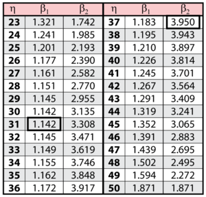
The solution is an iterative process that requires setting the value of [math]\displaystyle{ \beta\,\! }[/math] and finding the appropriate values of [math]\displaystyle{ \eta\,\! }[/math], and vice versa. The following table gives values of [math]\displaystyle{ \beta\,\! }[/math] based on given values of [math]\displaystyle{ \eta\,\! }[/math].

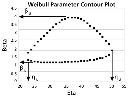
These data are represented graphically in the following contour plot:

(Note that this plot is generated with degrees of freedom [math]\displaystyle{ k = 1\,\! }[/math], as we are only determining bounds on one parameter. The contour plots generated in Weibull++ are done with degrees of freedom [math]\displaystyle{ k = 2\,\! }[/math], for use in comparing both parameters simultaneously.) As can be determined from the table, the lowest calculated value for [math]\displaystyle{ \beta\,\! }[/math] is 1.142, while the highest is 3.950. These represent the two-sided 90% confidence limits on this parameter. Since solutions for the equation do not exist for values of [math]\displaystyle{ \eta\,\! }[/math] below 23 or above 50, these can be considered the 90% confidence limits for this parameter. In order to obtain more accurate values for the confidence limits on [math]\displaystyle{ \eta\,\! }[/math], we can perform the same procedure as before, but finding the two values of [math]\displaystyle{ \eta\,\! }[/math] that correspond with a given value of [math]\displaystyle{ \beta\,\! }[/math] Using this method, we find that the 90% confidence limits on [math]\displaystyle{ \eta\,\! }[/math] are 22.474 and 49.967, which are close to the initial estimates of 23 and 50.

Note that the points where [math]\displaystyle{ \beta\,\! }[/math] are maximized and minimized do not necessarily correspond with the points where [math]\displaystyle{ \eta\,\! }[/math] are maximized and minimized. This is due to the fact that the contour plot is not symmetrical, so that the parameters will have their extremes at different points.

Likelihood Ratio Bounds on Time (Type I)

Likelihood Ratio Bounds on Time (Type I)

For the data given in Example 1, determine the 90% two-sided confidence bounds on the time estimate for a reliability of 50%. The ML estimate for the time at which [math]\displaystyle{ R(t)=50%\,\! }[/math] is 28.930.

Solution

In this example, we are trying to determine the 90% two-sided confidence bounds on the time estimate of 28.930. As was mentioned, we need to rewrite the likelihood ratio equation so that it is in terms of [math]\displaystyle{ t\,\! }[/math] and [math]\displaystyle{ \beta .\,\! }[/math] This is accomplished by using a form of the Weibull reliability equation, [math]\displaystyle{ R={{e}^{-{{\left( \tfrac{t}{\eta } \right)}^{\beta }}}}.\,\! }[/math] This can be rearranged in terms of [math]\displaystyle{ \eta \,\! }[/math], with [math]\displaystyle{ R\,\! }[/math] being considered a known variable or:

[math]\displaystyle{ \eta =\frac{t}{{{(-\text{ln}(R))}^{\tfrac{1}{\beta }}}}\,\! }[/math]

This can then be substituted into the [math]\displaystyle{ \eta \,\! }[/math] term in the likelihood ratio equation to form a likelihood equation in terms of [math]\displaystyle{ t\,\! }[/math] and [math]\displaystyle{ \beta \,\! }[/math] or:

[math]\displaystyle{ \begin{align} & L(\beta ,t)= & \underset{i=1}{\overset{N}{\mathop \prod }}\,f({{x}_{i}};\beta ,t,R) \\ & & \end{align}\,\! }[/math]

[math]\displaystyle{ =\underset{i=1}{\overset{5}{\mathop \prod }}\,\frac{\beta }{\left( \tfrac{t}{{{(-\text{ln}(R))}^{\tfrac{1}{\beta }}}} \right)}\cdot {{\left( \frac{{{x}_{i}}}{\left( \tfrac{t}{{{(-\text{ln}(R))}^{\tfrac{1}{\beta }}}} \right)} \right)}^{\beta -1}}\cdot \text{exp}\left[ -{{\left( \frac{{{x}_{i}}}{\left( \tfrac{t}{{{(-\text{ln}(R))}^{\tfrac{1}{\beta }}}} \right)} \right)}^{\beta }} \right]\,\! }[/math]

where [math]\displaystyle{ {{x}_{i}}\,\! }[/math] are the original time-to-failure data points. We can now rearrange the likelihood ratio equation to the form:

[math]\displaystyle{ L(\beta ,t)-L(\widehat{\beta },\widehat{\eta })\cdot {{e}^{\tfrac{-\chi _{\alpha ;1}^{2}}{2}}}=0\,\! }[/math]

Since our specified confidence level, [math]\displaystyle{ \delta \,\! }[/math], is 90%, we can calculate the value of the chi-squared statistic, [math]\displaystyle{ \chi _{0.9;1}^{2}=2.705543.\,\! }[/math] We can now substitute this information into the equation:

[math]\displaystyle{ \begin{align} L(\beta ,t)-L(\widehat{\beta },\widehat{\eta })\cdot {{e}^{\tfrac{-\chi _{\alpha ;1}^{2}}{2}}}= & 0 \\ \\ L(\beta ,t)-1.714714\times {{10}^{-9}}\cdot {{e}^{\tfrac{-2.705543}{2}}}= & 0 \\ & \\ L(\beta ,t)-4.432926\cdot {{10}^{-10}}= & 0 \end{align}\,\! }[/math]

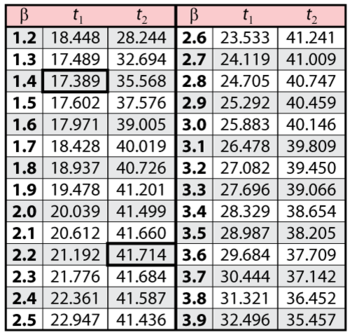
Note that the likelihood value for [math]\displaystyle{ L(\widehat{\beta },\widehat{\eta })\,\! }[/math] is the same as it was for Example 1. This is because we are dealing with the same data and parameter estimates or, in other words, the maximum value of the likelihood function did not change. It now remains to find the values of [math]\displaystyle{ \beta \,\! }[/math] and [math]\displaystyle{ t\,\! }[/math] which satisfy this equation. This is an iterative process that requires setting the value of [math]\displaystyle{ \beta \,\! }[/math] and finding the appropriate values of [math]\displaystyle{ t\,\! }[/math]. The following table gives the values of [math]\displaystyle{ t\,\! }[/math] based on given values of [math]\displaystyle{ \beta \,\! }[/math].

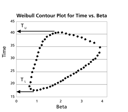
These points are represented graphically in the following contour plot:

As can be determined from the table, the lowest calculated value for [math]\displaystyle{ t\,\! }[/math] is 17.389, while the highest is 41.714. These represent the 90% two-sided confidence limits on the time at which reliability is equal to 50%.

Likelihood Ratio Bounds on Reliability (Type 2)

Likelihood Ratio Bounds on Reliability (Type 2)

For the data given in Example 1, determine the 90% two-sided confidence bounds on the reliability estimate for [math]\displaystyle{ t=45\,\! }[/math]. The ML estimate for the reliability at [math]\displaystyle{ t=45\,\! }[/math] is 14.816%.

Solution

In this example, we are trying to determine the 90% two-sided confidence bounds on the reliability estimate of 14.816%. As was mentioned, we need to rewrite the likelihood ratio equation so that it is in terms of [math]\displaystyle{ R\,\! }[/math] and [math]\displaystyle{ \beta .\,\! }[/math] This is again accomplished by substituting the Weibull reliability equation into the [math]\displaystyle{ \eta \,\! }[/math] term in the likelihood ratio equation to form a likelihood equation in terms of [math]\displaystyle{ R\,\! }[/math] and [math]\displaystyle{ \beta \,\! }[/math]:

[math]\displaystyle{ \begin{align} & L(\beta ,R)= & \underset{i=1}{\overset{N}{\mathop \prod }}\,f({{x}_{i}};\beta ,t,R) \\ & & \end{align}\,\! }[/math]

[math]\displaystyle{ =\underset{i=1}{\overset{5}{\mathop \prod }}\,\frac{\beta }{\left( \tfrac{t}{{{(-\text{ln}(R))}^{\tfrac{1}{\beta }}}} \right)}\cdot {{\left( \frac{{{x}_{i}}}{\left( \tfrac{t}{{{(-\text{ln}(R))}^{\tfrac{1}{\beta }}}} \right)} \right)}^{\beta -1}}\cdot \text{exp}\left[ -{{\left( \frac{{{x}_{i}}}{\left( \tfrac{t}{{{(-\text{ln}(R))}^{\tfrac{1}{\beta }}}} \right)} \right)}^{\beta }} \right]\,\! }[/math]

where [math]\displaystyle{ {{x}_{i}}\,\! }[/math] are the original time-to-failure data points. We can now rearrange the likelihood ratio equation to the form:

[math]\displaystyle{ L(\beta ,R)-L(\widehat{\beta },\widehat{\eta })\cdot {{e}^{\tfrac{-\chi _{\alpha ;1}^{2}}{2}}}=0\,\! }[/math]

Since our specified confidence level, [math]\displaystyle{ \delta \,\! }[/math], is 90%, we can calculate the value of the chi-squared statistic, [math]\displaystyle{ \chi _{0.9;1}^{2}=2.705543.\,\! }[/math] We can now substitute this information into the equation:

[math]\displaystyle{ \begin{align} L(\beta ,R)-L(\widehat{\beta },\widehat{\eta })\cdot {{e}^{\tfrac{-\chi _{\alpha ;1}^{2}}{2}}}= & 0 \\ \\ L(\beta ,R)-1.714714\times {{10}^{-9}}\cdot {{e}^{\tfrac{-2.705543}{2}}}= & 0 \\ \\ L(\beta ,R)-4.432926\cdot {{10}^{-10}}= & 0 \end{align}\,\! }[/math]

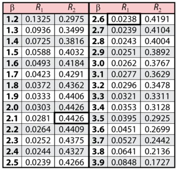
It now remains to find the values of [math]\displaystyle{ \beta \,\! }[/math] and [math]\displaystyle{ R\,\! }[/math] that satisfy this equation. This is an iterative process that requires setting the value of [math]\displaystyle{ \beta \,\! }[/math] and finding the appropriate values of [math]\displaystyle{ R\,\! }[/math]. The following table gives the values of [math]\displaystyle{ R\,\! }[/math] based on given values of [math]\displaystyle{ \beta \,\! }[/math].

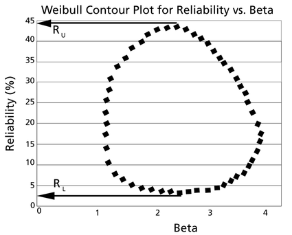
These points are represented graphically in the following contour plot:

As can be determined from the table, the lowest calculated value for [math]\displaystyle{ R\,\! }[/math] is 2.38%, while the highest is 44.26%. These represent the 90% two-sided confidence limits on the reliability at [math]\displaystyle{ t=45\,\! }[/math].

Comparing Parameter Estimation Methods Using Simulation Based Bounds

Comparing Parameter Estimation Methods Using Simulation Based Bounds

The purpose of this example is to determine the best parameter estimation method for a sample of ten units with complete time-to-failure data for each unit (i.e., no censoring). The data set follows a Weibull distribution with [math]\displaystyle{ \beta =2\,\! }[/math] and [math]\displaystyle{ \eta =100\,\! }[/math] hours.

The confidence bounds for the data set could be obtained by using Weibull++'s SimuMatic utility. To obtain the results, use the following settings in SimuMatic.

1. On the Main tab, choose the 2P-Weibull distribution and enter the given parameters (i.e., [math]\displaystyle{ \beta =2\,\! }[/math] and [math]\displaystyle{ \eta =100\,\! }[/math] hours)
2. On the Censoring tab, select the No censoring option.
3. On the Settings tab, set the number of data sets to 1,000 and the number of data points to 10.
4. On the Analysis tab, choose the RRX analysis method and set the confidence bounds to 90.

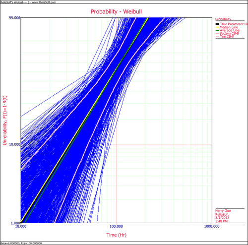
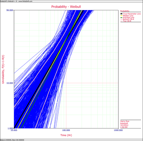
The following plot shows the simulation-based confidence bounds for the RRX parameter estimation method, as well as the expected variation due to sampling error.

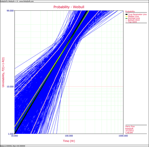
Create another SimuMatic folio and generate a second data using the same settings, but this time, select the RRY analysis method on the Analysis tab. The following plot shows the result.

The following plot shows the results using the MLE analysis method.

The results clearly demonstrate that the median RRX estimate provides the least deviation from the truth for this sample size and data type. However, the MLE outputs are grouped more closely together, as evidenced by the bounds.

This experiment can be repeated in SimuMatic using multiple censoring schemes (including Type I and Type II right censoring as well as random censoring) with various distributions. Multiple experiments can be performed with this utility to evaluate assumptions about the appropriate parameter estimation method to use for data sets.