Arrhenius Relationship: Difference between revisions
| Line 39: | Line 39: | ||
[[File:ALTA6.1.gif|400px]] | |||
::Figure 1: Graphical look at the Arrhenius life-stress relationship (linear scale) for a different life characteristics, assuming a Weibull distribution. | |||
Since the Arrhenius is a physics-based model derived for temperature dependence, it is used for temperature accelerated tests. For the same reason, temperature values must be in absolute units (Kelvin or Rankine), even though Eqn. (arrhenius) is unitless. | Since the Arrhenius is a physics-based model derived for temperature dependence, it is used for temperature accelerated tests. For the same reason, temperature values must be in absolute units (Kelvin or Rankine), even though Eqn. (arrhenius) is unitless. | ||
Revision as of 00:04, 28 July 2011
Introduction
The Arrhenius life-stress model (or relationship) is probably the most common life-stress relationship utilized in accelerated life testing. It has been widely used when the stimulus or acceleration variable (or stress) is thermal (i.e. temperature). It is derived from the Arrhenius reaction rate equation proposed by the Swedish physical chemist Svandte Arrhenius in 1887.
Formulation
The Arrhenius reaction rate equation is given by:
- where:
•
•
The activation energy is the energy that a molecule must have to participate in the reaction. In other words, the activation energy is a measure of the effect that temperature has on the reaction.
The Arrhenius life-stress model is formulated by assuming that life is proportional to the inverse reaction rate of the process, thus the Arrhenius life-stress relationship is given by:
- where:
•
•
•
•
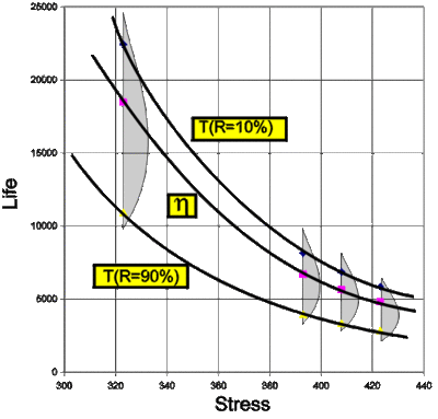
- Figure 1: Graphical look at the Arrhenius life-stress relationship (linear scale) for a different life characteristics, assuming a Weibull distribution.
Since the Arrhenius is a physics-based model derived for temperature dependence, it is used for temperature accelerated tests. For the same reason, temperature values must be in absolute units (Kelvin or Rankine), even though Eqn. (arrhenius) is unitless.
Life Stress Plots
The Arrhenius relationship can be linearized and plotted on a Life vs. Stress plot, also called the Arrhenius plot. The relationship is linearized by taking the natural logarithm of both sides in Eqn. (arrhenius) or:
In Eqn. (log-arrh)
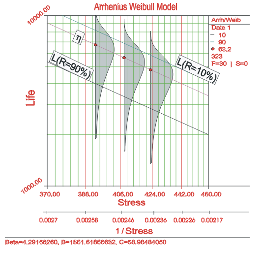
- Fig. 3: An illustration of both reciprocal and non-reciprocal scales.
The Arrhenius relationship is plotted on a reciprocal scale for practical reasons. For example, in Fig. 3 it is more convenient to locate the life corresponding to a stress level of 370K than to take the reciprocal of 370K (0.0027) first, and then locate the corresponding life.
The shaded areas shown in Fig. 3 are the imposed at each test stress level. From such imposed
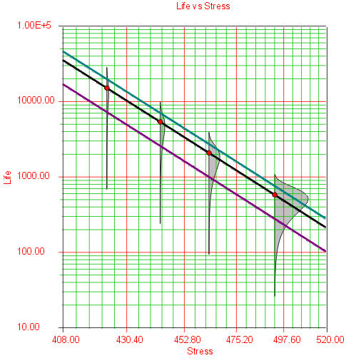
- Fig. 4: An example of scatter in life at each test stress level.
Activation Energy and the Parameter B
Depending on the application (and where the stress is exclusively thermal), the parameter
Note that in this formulation, the activation energy
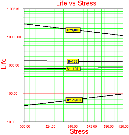
- Fig. 5: Behavior of the parameter B.
Acceleration Factor
Most practitioners use the term acceleration factor to refer to the ratio of the life (or acceleration characteristic) between the use level and a higher test stress level or:
For the Arrhenius model this factor is:
Thus, if
Arrhenius-Exponential
The
It can be easily shown that the mean life for the 1-parameter exponential distribution (presented in detail in Chapter 5) is given by:
thus:
The Arrhenius-exponential model
Therefore:
Substituting for
Arrhenius-Exponential Statistical Properties Summary
Mean or MTTF
The mean,
Median
The median,
Mode
The mode,
Standard Deviation
The standard deviation,
Arrhenius-Exponential Reliability Function
The Arrhenius-exponential reliability function is given by:
This function is the complement of the Arrhenius-exponential cumulative distribution function or:
and:
Conditional Reliability
The Arrhenius-exponential conditional reliability function is given by,
Reliable Life
For the Arrhenius-exponential model, the reliable life, or the mission duration for a desired reliability goal,
or:
Parameter Estimation
Maximum Likelihood Estimation Method
The log-likelihood function for the exponential distribution is as shown next:
where:
and:
•
Substituting the Arrhenius-exponential model into the log-likelihood function yields:
where:
The solution (parameter estimates) will be found by solving for the parameters
Arrhenius-Weibull
The
New format available! This reference is now available in a new format that offers faster page load, improved display for calculations and images, more targeted search and the latest content available as a PDF. As of September 2023, this Reliawiki page will not continue to be updated. Please update all links and bookmarks to the latest reference at help.reliasoft.com/reference/accelerated_life_testing_data_analysis
|
Chapter 4: Arrhenius Relationship |
Available Software: More Resources: |
Introduction
The Arrhenius life-stress model (or relationship) is probably the most common life-stress relationship utilized in accelerated life testing. It has been widely used when the stimulus or acceleration variable (or stress) is thermal (i.e. temperature). It is derived from the Arrhenius reaction rate equation proposed by the Swedish physical chemist Svandte Arrhenius in 1887.
Formulation
The Arrhenius reaction rate equation is given by:
- where:
•
•
The activation energy is the energy that a molecule must have to participate in the reaction. In other words, the activation energy is a measure of the effect that temperature has on the reaction.
The Arrhenius life-stress model is formulated by assuming that life is proportional to the inverse reaction rate of the process, thus the Arrhenius life-stress relationship is given by:
- where:
•
•
•
•
- Figure 1: Graphical look at the Arrhenius life-stress relationship (linear scale) for a different life characteristics, assuming a Weibull distribution.
Since the Arrhenius is a physics-based model derived for temperature dependence, it is used for temperature accelerated tests. For the same reason, temperature values must be in absolute units (Kelvin or Rankine), even though Eqn. (arrhenius) is unitless.
Life Stress Plots
The Arrhenius relationship can be linearized and plotted on a Life vs. Stress plot, also called the Arrhenius plot. The relationship is linearized by taking the natural logarithm of both sides in Eqn. (arrhenius) or:
In Eqn. (log-arrh)
- Fig. 3: An illustration of both reciprocal and non-reciprocal scales.
The Arrhenius relationship is plotted on a reciprocal scale for practical reasons. For example, in Fig. 3 it is more convenient to locate the life corresponding to a stress level of 370K than to take the reciprocal of 370K (0.0027) first, and then locate the corresponding life.
The shaded areas shown in Fig. 3 are the imposed at each test stress level. From such imposed
- Fig. 4: An example of scatter in life at each test stress level.
Activation Energy and the Parameter B
Depending on the application (and where the stress is exclusively thermal), the parameter
Note that in this formulation, the activation energy
- Fig. 5: Behavior of the parameter B.
Acceleration Factor
Most practitioners use the term acceleration factor to refer to the ratio of the life (or acceleration characteristic) between the use level and a higher test stress level or:
For the Arrhenius model this factor is:
Thus, if
Arrhenius-Exponential
The
It can be easily shown that the mean life for the 1-parameter exponential distribution (presented in detail in Chapter 5) is given by:
thus:
The Arrhenius-exponential model
Therefore:
Substituting for
Arrhenius-Exponential Statistical Properties Summary
Mean or MTTF
The mean,
Median
The median,
Mode
The mode,
Standard Deviation
The standard deviation,
Arrhenius-Exponential Reliability Function
The Arrhenius-exponential reliability function is given by:
This function is the complement of the Arrhenius-exponential cumulative distribution function or:
and:
Conditional Reliability
The Arrhenius-exponential conditional reliability function is given by,
Reliable Life
For the Arrhenius-exponential model, the reliable life, or the mission duration for a desired reliability goal,
or:
Parameter Estimation
Maximum Likelihood Estimation Method
The log-likelihood function for the exponential distribution is as shown next:
where:
and:
•
Substituting the Arrhenius-exponential model into the log-likelihood function yields:
where:
The solution (parameter estimates) will be found by solving for the parameters
Arrhenius-Weibull
The
- Template loop detected: Template:Weibull2pdf
The scale parameter (or characteristic life) of the Weibull distribution is
The Arrhenius-Weibull model pdf can then be obtained by setting
and substituting for
An illustration of the
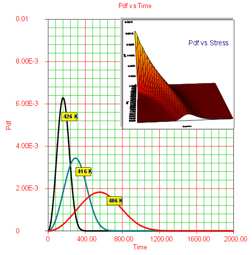
- Fig. 6: Behavior of the probability density function at different stresses and with the parameters held constant.
The advantage of using the Weibull distribution as the life distribution lies in its flexibility to assume different shapes. The Weibull distribution is presented in greater detail in Chapter 5.
Arrhenius-Weibull Statistical Properties Summary
Mean or MTTF
The mean,
where
Median
The median,
Mode
The mode,
Standard Deviation
The standard deviation,
Arrhenius-Weibull Reliability Function
The Arrhenius-Weibull reliability function is given by:
If the parameter
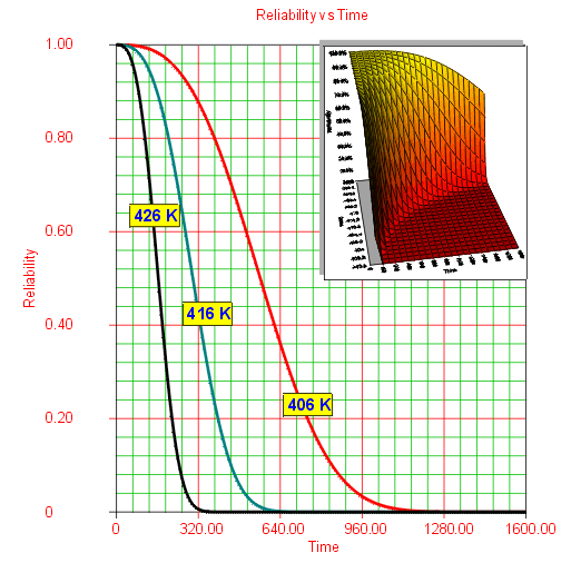
- Fig. 7: Behavior of the reliability function at different stress and constant parameter values.
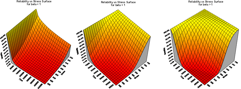
The behavior of the reliability function of the Weibull distribution for different values of
- Fig. 8: Reliability function for
- Fig. 8: Reliability function for
Conditional Reliability Function
The Arrhenius-Weibull conditional reliability function at a specified stress level is given by:
or:
Reliable Life
For the Arrhenius-Weibull relationship, the reliable life,
This is the life for which the unit will function successfully with a reliability of
Arrhenius-Weibull Failure Rate Function
The Arrhenius-Weibull failure rate function,
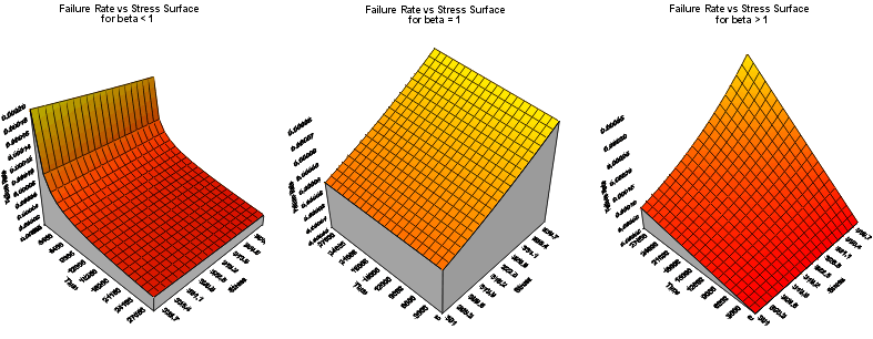
- Fig. 9: Failure rate function for
- Fig. 9: Failure rate function for
Parameter Estimation
Maximum Likelihood Estimation Method
The Arrhenius-Weibull log-likelihood function is as follows:
where:
and:
•
Example
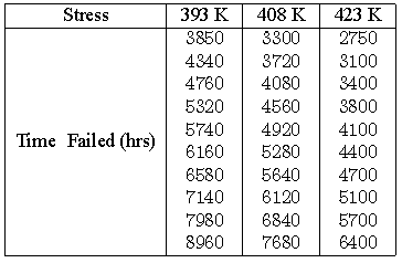
Consider the following times-to-failure data at three different stress levels.
The data set was analyzed jointly and with a complete MLE solution over the entire data set, using ReliaSoft's ALTA. The analysis yields:
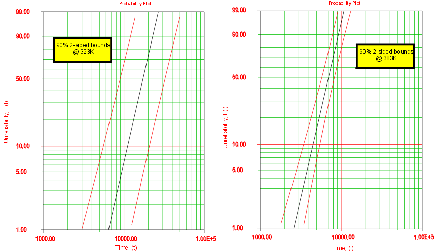
Once the parameters of the model are estimated, extrapolation and other life measures can be directly obtained using the appropriate equations. Using the MLE method, confidence bounds for all estimates can be obtained. Note in Fig. 10 that the more distant the accelerated stress from the operating stress, the greater the uncertainty of the extrapolation. The degree of uncertainty is reflected in the confidence bounds. (General theory and calculations for confidence intervals are presented in Appendix A. Specific calculations for confidence bounds on the Arrhenius model are presented in Appendix 6.A following this chapter.)
- Fig. 10: Comparison of the confidence bounds for different use stress levels.
Arrhenius-Lognormal
The
where:
and:
•
The median of the lognormal distribution is given by:
The Arrhenius-lognormal model
or:
Thus:
Substituting Eqn. (arrh-logn-mean) into Eqn. (arrh-logn-pdf) yields the Arrhenius-lognormal model
Note that in Eqn. (arrh-logn-pdf), it was assumed that the standard deviation of the natural logarithms of the times-to-failure,
Arrhenius-Lognormal Statistical Properties Summary
The Mean
• The mean life of the Arrhenius-lognormal model (mean of the times-to-failure),
• The mean of the natural logarithms of the times-to-failure,
The Standard Deviation
• The standard deviation of the Arrhenius-lognormal model (standard deviation of the times-to-failure),
• The standard deviation of the natural logarithms of the times-to-failure,
The Mode
• The mode of the Arrhenius-lognormal model is given by:
Arrhenius-Lognormal Reliability Function
The reliability for a mission of time
vor:
There is no closed form solution for the lognormal reliability function. Solutions can be obtained via the use of standard normal tables. Since the application automatically solves for the reliability, we will not discuss manual solution methods.
Reliable Life
For the Arrhenius-lognormal model, the reliable life, or the mission duration for a desired reliability goal,
where:
and:
Since
Arrhenius-Lognormal Failure Rate
The Arrhenius-lognormal failure rate is given by:
When Using the Lognormal Distribution in ALTA
The parameters returned for the Arrhenius-lognormal distribution are always
Parameter Estimation
Maximum Likelihood Estimation Method
The lognormal log-likelihood function for the Arrhenius-lognormal model is as follows:
where:
and:
•
and:
Appendix 6.A: Arrhenius Confidence Bounds
Approximate Confidence Bounds for the Arrhenius-Exponential
There are different methods for computing confidence bounds. ALTA utilizes confidence bounds that are based on the asymptotic theory for maximum likelihood estimates, most commonly referred to as the Fisher matrix bounds.
Confidence Bounds on the Mean Life
The Arrhenius-exponential distribution is given by Eqn. (arrhenius) by setting
where
If
or:
The variances and covariance of
Confidence Bounds on Reliability
The bounds on reliability for any given time,
where
Confidence Bounds on Time
The bounds on time (ML estimate of time) for a given reliability are estimated by first solving the reliability function with respect to time:
The corresponding confidence bounds are then estimated from:
where
Approximate Confidence Bounds for the Arrhenius-Weibull:
Bounds on the Parameters
From the asymptotically normal property of the maximum likelihood estimators, and since
also:
and:
The variances and covariances of
Confidence Bounds on Reliability
The reliability function for the Arrhenius-Weibull model (ML estimate) is given by:
or:
Setting:
or:
The reliability function now becomes:
The next step is to find the upper and lower bounds on
where:
or:
The upper and lower bounds on reliability are:
where
Confidence Bounds on Time
The bounds on time for a given reliability are estimated by first solving the reliability function with respect to time:
or:
where
The upper and lower bounds on
where:
or:
The upper and lower bounds on time can then found by:
where
Approximate Confidence Bounds for the Arrhenius-Lognormal
Bounds on the Parameters
The lower and upper bounds on
Since the standard deviation,
and:
The variances and covariances of
Bounds on Reliability
The reliability of the lognormal distribution is:
Let
The bounds on
where:
or:
The upper and lower bounds on reliability are:
Confidence Bounds on Time
The bounds around time, for a given lognormal percentile (unreliability), are estimated by first solving the reliability equation with respect to time, as follows:
where:
and:
The next step is to calculate the variance of
or:
The upper and lower bounds are then found by:
Solving for
| The material on this page is copyrighted. | ©1992-2012. ReliaSoft Corporation. ALL RIGHTS RESERVED. |

