Imperfect Repairs

This article also appears in the System Analysis Reference book.

Restoration Factors (RF)

The concept of a restoration factor may be used in cases in which one wants to model imperfect repair, or a repair with a used component. The best way to indicate that a component is not as good as new is to give the component some age. As an example, if one is dealing with car tires, a tire that is not as good as new would have some pre-existing wear on it. In other words, the tire would have some accumulated mileage. A restoration factor concept is used to better describe the existing age of a component. The restoration factor is used to determine the age of the component after a repair or any other maintenance action (addressed in later sections, such as a PM action or inspection).

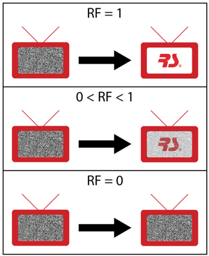
The restoration factor in BlockSim is defined as a number between 0 and 1 and has the following effect:

1. A restoration factor of 1 (100%) implies that the component is as good as new after repair, which in effect implies that the starting age of the component is 0.
2. A restoration factor of 0 implies that the component is the same as it was prior to repair, which in effect implies that the starting age of the component is the same as the age of the component at failure.
3. A restoration factor of 0.25 (25%) implies that the starting age of the component is equal to 75% of the age of the component at failure.
   

The figure below provides a visual demonstration of restoration factors. It should be noted that for successive maintenance actions on the same component, the age of the component after such an action is the initial age plus the time to failure since the last maintenance action.

Type I and Type II RFs

BlockSim offers two kinds of restoration factors. The type I restoration factor is based on Kijima [12, 13] model I and assumes that the repairs can only fix the wear-out and damage incurred during the last period of operation. Thus, the nth repair can only remove the damage incurred during the time between the (n-1)th and nth failures. The type II restoration factor, based on Kijima model II, assumes that the repairs fix all of the wear-out and damage accumulated up to the current time. As a result, the nth repair not only removes the damage incurred during the time between the (n-1)th and nth failures, but can also fix the cumulative damage incurred during the time from the first failure to the (n-1)th failure.

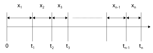
To illustrate this, consider a repairable system, observed from time [math]\displaystyle{ t=0\,\! }[/math], as shown in figure above. Let the successive failure times be denoted by [math]\displaystyle{ {{t}_{1}}\,\! }[/math], [math]\displaystyle{ {{t}_{2}}\,\! }[/math], ... and let the times between failures be denoted by [math]\displaystyle{ {{x}_{1}}\,\! }[/math], [math]\displaystyle{ {{x}_{2}}\,\! }[/math], .... Let [math]\displaystyle{ RF\,\! }[/math] denote the restoration factor, then the age of the system [math]\displaystyle{ {{v}_{n}}\,\! }[/math] at time [math]\displaystyle{ {{t}_{n}}\,\! }[/math] using the two types of restoration factors is:

Type I Restoration Factor:

[math]\displaystyle{ \begin{align} {{v}_{n}}={{v}_{n-1}}+(1-RF){{x}_{n}} \end{align}\,\! }[/math]

Type II Restoration Factor:

[math]\displaystyle{ \begin{align} {{v}_{n}}=(1-RF)({{v}_{n-1}}+{{x}_{n}}) \end{align}\,\! }[/math]

Illustrating Type I RF Through an Example

Assume that you have a component with a Weibull failure distribution ([math]\displaystyle{ \beta\,\! }[/math] = 1.5, [math]\displaystyle{ \eta\,\! }[/math] = 1000 hours), RF type I = 0.25 and the component undergoes instant repair. Furthermore, assume that the component starts life new (i.e., with a start age of zero). The simulation steps are as follows:

1. Generate a uniform random number, [math]\displaystyle{ {{U}_{R}}[0,1] = 0.7021885\,\! }[/math].
   
2. Then, the first failure event will be at 500 hours.
   
3. After instantaneous repair, the component will begin life with an age after repair of 375 hours [math]\displaystyle{ ((1-0.25) \times 500)\,\! }[/math].
   
4. Generate another uniform random number, [math]\displaystyle{ {{U}_{R}}[0,1] = 0.8824969\,\! }[/math].
   
5. The next failure event is now determined using the conditional reliability equation, or:
   

[math]\displaystyle{ \begin{align} R(x+v)= & R(x,v)\cdot R(v) \\ R(x+375)= & 0.8824969\cdot R(375) \\ R(x+375)= & 0.8824969\cdot 0.7948200 \\ R(x+375)= & 0.7014261 \\ x+375= & 501.024 \\ x = & 126.024 \end{align}\,\! }[/math]

Thus, the next failure event will be at 500 + 126.024 = 626.024 hours. Note that if the component had been as good as new (i.e., RF = 100%), then the next failure would have been at 750 hours (500 + 250), where 250 hours is the time corresponding to a reliability of 0.8824969, which is the random number that was generated in Step 4.

6. At this failure point, the item's age will now be equal to the initial age, after the first corrective action, plus the additional time it operated, or 375 + 126.024 = 501.024 hours.

7. Thus, the age after the second repair will be the sum of the previous age and the restoration factor times the age of the component since the last failure, or 375 + ((1-0.25) x 126.024) = 469.518 hours.

8. Go to Step 4 and repeat the process.

Illustrating Type II RF Through an Example

Assume that you have a component with a Weibull failure distribution ([math]\displaystyle{ \beta\,\! }[/math] = 1.5, [math]\displaystyle{ \eta\,\! }[/math] = 1000 hours), RF type II = 0.25 and the component undergoes instant repair. Furthermore, assume that the component starts life new (i.e., with a start age of zero). The simulation steps are as follows:

1. Generate a uniform random number, [math]\displaystyle{ {{U}_{R}}[0,1] = 0.7021885\,\! }[/math].
   
2. Then, the first failure event will be at 500 hours.
   
3. After instantaneous repair, the component will begin life with an age after repair of 375 hours ((1 - 0.25) x 500).
   
4. Generate another uniform random number, [math]\displaystyle{ {{U}_{R}}[0,1] = 0.8824969\,\! }[/math].
   

1. The next failure event is now determined using the conditional reliability equation, or:

[math]\displaystyle{ \begin{align} R(x+v)= & R(x,v)\cdot R(v) \\ R(x+375)= & 0.8824969\cdot R(375) \\ R(x+375)= & 0.8824969\cdot 0.7948200 \\ R(x+375)= & 0.7014261 \\ x+375= & 501.024 \\ x= & 126.024 \end{align}\,\! }[/math]

Thus, the next failure event will be at 500 + 126.024 = 626.024 hours. Note that if the component had been as good as new (i.e., RF = 100%), then the next failure would have been at 750 hours (500 + 250), where 250 is the time corresponding to a reliability of 0.8824969, which is the random number that was generated in Step 4.

6. At this failure point, the item's age will now be equal to the initial age, after the first corrective action, plus the additional time it operated, or 375 + 126.024 = 501.024 hours.

7. Thus, the age after the second repair will be the restoration factor times the age of the component at failure, or (1 - 0.25) x (375 + 126.024) = 375.768 hours.

8. Go to Step 4 and repeat the process.

Discussion of Type I and Type II RFs

As an application example, consider an automotive engine that fails after six years of operation. The engine is rebuilt. The rebuild has the effect of rejuvenating the engine to a condition as if it were three years old (i.e., a 50% RF). Assume that the rebuild affects all of the damage on the engine (i.e., a Type II restoration). The engine fails again after three years (when it again reaches an age of six) and another rebuild is required. This rebuild will also rejuvenate the engine by 50%, thus making it three years old again.

Now consider a similar engine subjected to a similar rebuild, but that the rebuild only affects the damage since the last repair (i.e., a Type I restoration of 50%). The first rebuild will rejuvenate the engine to a three-year-old condition. The engine will fail again after three years, but the rebuild this time will only affect the age (of three years) after the first rebuild. Thus the engine will have an age of four and a half years after the second rebuild ( [math]\displaystyle{ 3+(1-0.5) \times 3=4.5\,\! }[/math] ). After the second rebuild the engine will fail again after a period of one and a half years and a third rebuild will be required. The age of the engine after the third rebuild will be five years and three months ( [math]\displaystyle{ 4.5+(1-0.5) \times 1.5=5.25\,\! }[/math] ).

It should be pointed out that when dealing with constant failure rates (i.e., with a distribution such as the exponential), the restoration factor has no effect.

Calculations to Obtain RFs

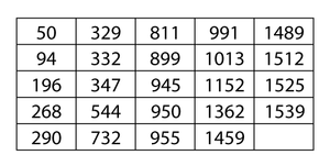
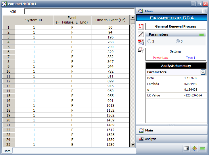
The two types of restoration factors discussed in the previous sections can be calculated using the parametric RDA (Recurrent Data Analysis) tool in Weibull++. This tool uses the GRP (General Renewal Process) model to analyze failure data of a repairable item. More information on the Parametric RDA tool and the GRP (General Renewal Process) model can be found in [25]. As an example, consider the times to failure for an air-conditioning unit of an aircraft recorded in the following table. Assume that each time the unit is repaired, the repair can only remove the damage incurred during the last period of operation. This assumption implies a type I RF factor which is specified as an analysis setting in the Weibull++ folio. The type I RF for the air-conditioning unit can be calculated using the results from Weibull++ shown in the figure below.

Using the Parametric RDA tool in Weibull++ to calculate restoration factors.

The value of the action effectiveness factor [math]\displaystyle{ q\,\! }[/math] obtained from Weibull++ is:

[math]\displaystyle{ \begin{align} q=0.1344 \end{align}\,\! }[/math]

The type I RF factor is calculated using [math]\displaystyle{ q\,\! }[/math] as:

[math]\displaystyle{ \begin{align} RF= & 1-q \\ = & 1-0.1344 \\ = & 0.8656 \end{align}\,\! }[/math]

The parameters of the Weibull distribution for the air-conditioning unit can also be calculated. [math]\displaystyle{ \beta \,\! }[/math] is obtained from Weibull++ as 1.1976. [math]\displaystyle{ \eta \,\! }[/math] can be calculated using the [math]\displaystyle{ \beta \,\! }[/math] and [math]\displaystyle{ \lambda \,\! }[/math] values from Weibull++ as:

[math]\displaystyle{ \begin{align} \eta = & {{\left( \frac{1}{\lambda } \right)}^{\tfrac{1}{\beta }}} \\ = & {{\left( \frac{1}{0.0049} \right)}^{\tfrac{1}{1.1976}}} \\ = & 84.8582 \end{align}\,\! }[/math]

The values of the type I RF, [math]\displaystyle{ \beta \,\! }[/math] and [math]\displaystyle{ \eta \,\! }[/math] calculated above can now be used to model the air-conditioning unit as a component in BlockSim.