Difference Detection Matrix Example

Test Design Using Life Difference Detection Matrix

Assume there are two design options for a new product. Engineers need to design a test to compare the reliability performance of these two options. The reliability for both designs is assumed to follow a Weibull distribution. For Design 1, its shape parameter [math]\displaystyle{ β }[/math] = 3; for Design 2, its [math]\displaystyle{ β }[/math] = 2. Their B10 lives may range from 500 to 3,000 hours. We want to use the Difference Detection Matrix to choose the suitable sample size and test duration.

Solution

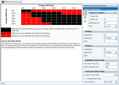
Initially, the sample size for each design is set to 20. Two test durations of 3,000 and 5,000 hours also were chosen. Based on these settings and the assumptions on the failure time distributions, the following Difference Detection Matrix is obtained.

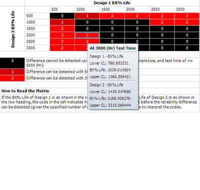
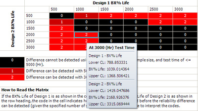
In the figure, the range of the assumed B10 life for each design is from 500 to 3,000 hours. The pair-wised comparison results are displayed in each cell. 0 means the difference cannot be detected through the test; 1 means the difference can be detected if the test duration is 5,000 hours; 2 means the difference can be detected if the test duration is 3,000 hours. For example, the number is 2 for for cell (1000, 2000). This means that if the B10 life for Design 1 is 1,000 hours and the B10 life for Design 2 is 2,000 hours, the difference can be detected if the test duration is at least 5,000 hours. By testing 20 samples each for 3,000 hours, the difference of their B10 lives probably can be detected. This is because, at a confidence level of 90%, the estimated confidence intervals on the B10 life do not overlap. The estimated intervals can be seen in the figure below.

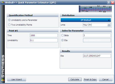
We will use Design 1 to illustrate how the interval is calculated. For cell (1000, 2000), Design 1's B10 life is 1,000 and the assumed [math]\displaystyle{ β }[/math] is 3. We can calculate the [math]\displaystyle{ η }[/math] for the Weibull distribution using the Quick Parameter Estimator tool to calculate eta, as shown next.

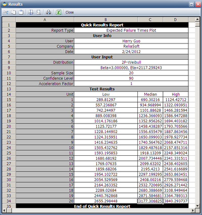
The estimated [math]\displaystyle{ η }[/math] is 2117.2592 hours. Then we can use these distribution parameters and the sample size of 20 to get the expected failure times using the Expected Failure Times Plot as shown below.

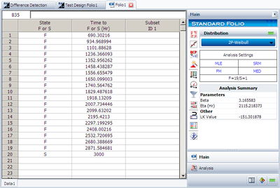
The median failure times are used to estimate the failure distribution. Please notice that since the test duration is set to 3,000 hours, any failures that occur after 3,000 are treated as suspensions. In this case, the last failure is a suspension with suspension time of 3,000. Now we can enter this data set into a standard Weibull++ folio as given in the next figure.

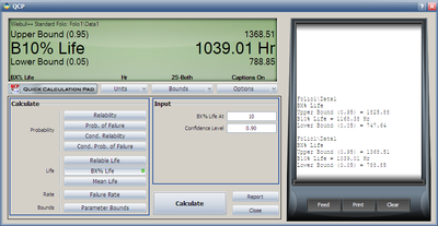
Please make sure the MLE and FM options are selected. Using the estimated results, we can calculate the B10 life and its interval in the QCP, as shown below.

From the above result, we can see the estimated B10 life and its confidence intervals are the same as the results displayed in the Difference Detection Matrix.

The above procedure can be repeated to get the results for the other cells and for Design 2. Therefore, by adjusting the sample size and test duration, a suitable test time can be identified for detecting a certain amount of difference between two designs/populations.