Warranty Data Analysis Dates Format Example: Difference between revisions
No edit summary |
Lisa Hacker (talk | contribs) No edit summary |
||
| (3 intermediate revisions by 2 users not shown) | |||
| Line 1: | Line 1: | ||
<noinclude>{{Banner Weibull Examples}}</noinclude> | <noinclude>{{Banner Weibull Examples}} | ||
''This example appears in the [https://help.reliasoft.com/reference/life_data_analysis Life data analysis reference]''. | |||
</noinclude> | |||
'''Dates of Failure Warranty Analysis''' | '''Dates of Failure Warranty Analysis''' | ||
Assume that a company has the following information for a product. | Assume that a company has the following information for a product. | ||
{| | border="1" align="center" style="border-collapse: collapse;" cellpadding="5" cellspacing="5" | |||
{| | border="1" | |||
|+ '''Sales''' | |+ '''Sales''' | ||
|- | |- | ||
| Line 53: | Line 55: | ||
{| | border="1" | {| | border="1" align="center" style="border-collapse: collapse;" cellpadding="5" cellspacing="5" | ||
|+ '''Returns''' | |+ '''Returns''' | ||
|- | |- | ||
| Line 98: | Line 100: | ||
{| | border="1" | {| | border="1" align="center" style="border-collapse: collapse;" cellpadding="5" cellspacing="5" | ||
| align="center" style="background:#f0f0f0;"|'''Quantity In-Service''' | | align="center" style="background:#f0f0f0;"|'''Quantity In-Service''' | ||
| align="center" style="background:#f0f0f0;"|'''Date In-Service''' | | align="center" style="background:#f0f0f0;"|'''Date In-Service''' | ||
| Line 114: | Line 116: | ||
|} | |} | ||
Using the given information to estimate the failure distribution of the product and forecast warranty returns. | Using the given information to estimate the failure distribution of the product and forecast warranty returns. | ||
'''Solution''' | '''Solution''' | ||
Create a warranty analysis folio using the dates of failure format. Enter the data from the tables in the '''Sales''', '''Returns''' and '''Future Sales''' sheets. On the control panel, click the '''Auto-Set''' button to automatically set the end date to the last day the warranty data were collected (September 14, 2011). Analyze the data using the 2P-Weibull distribution and RRX analysis method. The parameters are estimated to be beta = 1.315379 and eta = 102,381.486165. | Create a warranty analysis folio using the dates of failure format. Enter the data from the tables in the '''Sales''', '''Returns''' and '''Future Sales''' sheets. On the control panel, click the '''Auto-Set''' button to automatically set the end date to the last day the warranty data were collected (September 14, 2011). Analyze the data using the 2P-Weibull distribution and RRX analysis method. The parameters are estimated to be beta = 1.315379 and eta = 102,381.486165. | ||
The warranty folio automatically converts the warranty data into a format that can be used in a Weibull++ standard folio. To see this result, click anywhere within the '''Analysis Summary''' area of the control panel to open a report, as shown next (showing only the first 35 rows of data). In this example, rows 23 to 60 show the time-to-failure data that resulted from the conversion. | The warranty folio automatically converts the warranty data into a format that can be used in a Weibull++ standard folio. To see this result, click anywhere within the '''Analysis Summary''' area of the control panel to open a report, as shown next (showing only the first 35 rows of data). In this example, rows 23 to 60 show the time-to-failure data that resulted from the conversion. | ||
[[image:Warranty Dates Format Summary.png|center|500px]] | |||
[[image:Warranty Dates Format Summary.png | |||
To generate a forecast, click the '''Forecast''' icon on the control panel. In the Forecast Setup window, set the forecast to start on '''September 2011''' and set the number of forecast periods to '''6'''. Set the increment (length of each period) to '''1 Month''', as shown next. | To generate a forecast, click the '''Forecast''' icon on the control panel. In the Forecast Setup window, set the forecast to start on '''September 2011''' and set the number of forecast periods to '''6'''. Set the increment (length of each period) to '''1 Month''', as shown next. | ||
[[image:Warranty Dates Format Forecast Window.png|center|400px]] | |||
[[image:Warranty Dates Format Forecast Window.png | |||
Click '''OK'''. A Forecast sheet will be created, with the predicted future returns. Note that the first forecast will start on September 15, 2011 because the end of observation period was set to September 14, 2011. | Click '''OK'''. A Forecast sheet will be created, with the predicted future returns. Note that the first forecast will start on September 15, 2011 because the end of observation period was set to September 14, 2011. | ||
Click the '''Plot''' icon and choose the '''Expected Failures''' plot. The plot displays the predicted number of returns for each month, as shown next. | Click the '''Plot''' icon and choose the '''Expected Failures''' plot. The plot displays the predicted number of returns for each month, as shown next. | ||
[[image:Warranty Dates Format Predicted Failures Plot.png|center|600px]] | |||
[[image:Warranty Dates Format Predicted Failures Plot.png | |||
Latest revision as of 18:54, 18 September 2023
 |
New format available! This reference is now available in a new format that offers faster page load, improved display for calculations and images and more targeted search.
As of January 2024, this Reliawiki page will not continue to be updated. Please update all links and bookmarks to the latest references at Weibull examples and Weibull reference examples.
This example appears in the Life data analysis reference.
Dates of Failure Warranty Analysis
Assume that a company has the following information for a product.
| Quantity In-Service | Date In-Service |
| 6316 | 1/1/2010 |
| 8447 | 2/1/2010 |
| 5892 | 3/1/2010 |
| 596 | 4/1/2010 |
| 996 | 5/1/2010 |
| 8977 | 6/1/2010 |
| 2578 | 7/1/2010 |
| 8318 | 8/1/2010 |
| 2667 | 9/1/2010 |
| 7452 | 10/1/2010 |
| 1533 | 11/1/2010 |
| 9393 | 12/1/2010 |
| 1966 | 1/1/2011 |
| 8960 | 2/1/2011 |
| 6341 | 3/1/2011 |
| 4005 | 4/1/2011 |
| 3784 | 5/1/2011 |
| 5426 | 6/1/2011 |
| 4958 | 7/1/2011 |
| 6981 | 8/1/2011 |
| Quantity Returned | Date of Return | Date In-Service |
| 2 | 10/29/2010 | 10/1/2010 |
| 1 | 11/13/2010 | 10/1/2010 |
| 2 | 3/15/2011 | 10/1/2010 |
| 5 | 4/10/2011 | 10/1/2010 |
| 1 | 11/13/2010 | 11/1/2010 |
| 2 | 2/19/2011 | 11/1/2010 |
| 1 | 3/11/2011 | 11/1/2010 |
| 2 | 5/18/2011 | 11/1/2010 |
| 1 | 1/9/2011 | 12/1/2010 |
| 2 | 2/13/2011 | 12/1/2010 |
| 1 | 3/2/2011 | 12/1/2010 |
| 1 | 6/7/2011 | 12/1/2010 |
| 1 | 4/28/2011 | 1/1/2011 |
| 2 | 6/15/2011 | 1/1/2011 |
| 3 | 7/15/2011 | 1/1/2011 |
| 1 | 8/10/2011 | 2/1/2011 |
| 1 | 8/12/2011 | 2/1/2011 |
| 1 | 8/14/2011 | 2/1/2011 |
| Quantity In-Service | Date In-Service |
| 5000 | 9/1/2011 |
| 5000 | 10/1/2011 |
| 5000 | 11/1/2011 |
| 5000 | 12/1/2011 |
| 5000 | 1/1/2012 |
Using the given information to estimate the failure distribution of the product and forecast warranty returns.
Solution
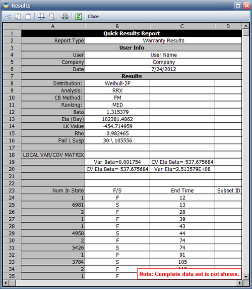
Create a warranty analysis folio using the dates of failure format. Enter the data from the tables in the Sales, Returns and Future Sales sheets. On the control panel, click the Auto-Set button to automatically set the end date to the last day the warranty data were collected (September 14, 2011). Analyze the data using the 2P-Weibull distribution and RRX analysis method. The parameters are estimated to be beta = 1.315379 and eta = 102,381.486165.
The warranty folio automatically converts the warranty data into a format that can be used in a Weibull++ standard folio. To see this result, click anywhere within the Analysis Summary area of the control panel to open a report, as shown next (showing only the first 35 rows of data). In this example, rows 23 to 60 show the time-to-failure data that resulted from the conversion.

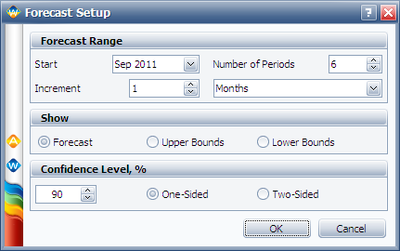
To generate a forecast, click the Forecast icon on the control panel. In the Forecast Setup window, set the forecast to start on September 2011 and set the number of forecast periods to 6. Set the increment (length of each period) to 1 Month, as shown next.

Click OK. A Forecast sheet will be created, with the predicted future returns. Note that the first forecast will start on September 15, 2011 because the end of observation period was set to September 14, 2011.
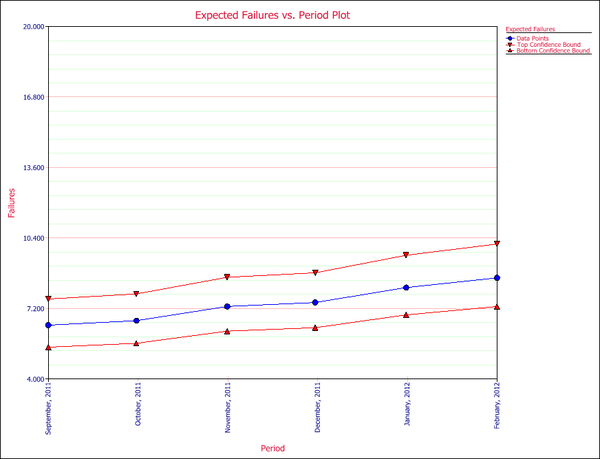
Click the Plot icon and choose the Expected Failures plot. The plot displays the predicted number of returns for each month, as shown next.
