|
|
| Line 32: |
Line 32: |
|
| |
|
| [[Image:Normal MLE Plot.png|thumb|center|400px| ]] | | [[Image:Normal MLE Plot.png|thumb|center|400px| ]] |
|
| |
| '''Special Note About Bias'''
| |
|
| |
| Estimators (i.e. parameter estimates) have properties such as unbiasedness, minimum variance, sufficiency, consistency, squared error constancy, efficiency and completeness [[Appendix: Weibull References|[7][5]]]. Numerous books and papers deal with these properties and this coverage is beyond the scope of this reference.
| |
|
| |
| However, we would like to briefly address one of these properties, unbiasedness. An estimator is said to be unbiased if the estimator <math>\widehat{\theta }=d({{X}_{1,}}{{X}_{2,}}...,{{X}_{n)}}</math> satisfies the condition <math>E\left[ \widehat{\theta } \right]</math> <math>=\theta </math> for all <math>\theta \in \Omega .</math>
| |
|
| |
| Note that <math>E\left[ X \right]</math> denotes the expected value of X and is defined (for continuous distributions) by:
| |
|
| |
| ::<math>\begin{align}
| |
| E\left[ X \right]= \int_{\varpi }x\cdot f(x)dx \\
| |
| X\in & \varpi .
| |
| \end{align}</math>
| |
|
| |
|
| |
| It can be shown [[Appendix: Weibull References|[7][5]]] that the MLE estimator for the mean of the normal (and lognormal) distribution does satisfy the unbiasedness criteria, or <math>E\left[ \widehat{\mu } \right]</math> <math>=\mu .</math> The same is not true for the estimate of the variance <math>\hat{\sigma }^{2}</math> . The maximum likelihood estimate for the variance for the normal distribution is given by:
| |
|
| |
| ::<math>\hat{\sigma }^{2}=\frac{1}{N}\underset{i=1}{\overset{N}{\mathop \sum }}\,{{({{t}_{i}}-\bar{T})}^{2}}</math>
| |
|
| |
| with a standard deviation of:
| |
|
| |
| ::<math>{{\hat{\sigma }}}=\sqrt{\frac{1}{N}\underset{i=1}{\overset{N}{\mathop \sum }}\,{{({{t}_{i}}-\bar{T})}^{2}}}</math>
| |
|
| |
|
| |
| These estimates, however, have been shown to be biased. It can be shown [[Appendix: Weibull References|[7][5]]] that the unbiased estimate of the variance and standard deviation for complete data is given by:
| |
|
| |
|
| |
| ::<math>\begin{align}
| |
| \hat{\sigma }^{2}= & \left[ \frac{N}{N-1} \right]\cdot \left[ \frac{1}{N}\underset{i=1}{\overset{N}{\mathop \sum }}\,{{({{t}_{i}}-\bar{T})}^{2}} \right]=\frac{1}{N-1}\underset{i=1}{\overset{N}{\mathop \sum }}\,{{({{t}_{i}}-\bar{T})}^{2}} \\
| |
| {{{\hat{\sigma }}}}= & \sqrt{\left[ \frac{N}{N-1} \right]\cdot \left[ \frac{1}{N}\underset{i=1}{\overset{N}{\mathop \sum }}\,{{({{t}_{i}}-\bar{T})}^{2}} \right]} \\
| |
| = & \sqrt{\frac{1}{N-1}\underset{i=1}{\overset{N}{\mathop \sum }}\,{{({{t}_{i}}-\bar{T})}^{2}}}
| |
| \end{align}</math>
| |
|
| |
|
| |
| Note that for larger values of <math>N</math> , <math>\sqrt{\left[ N/(N-1) \right]}</math> tends to 1.
| |
|
| |
| The Use Unbiased Std on Normal Data option in the User Setup under the Calculations tab allows biasing to be considered when estimating the parameters.
| |
|
| |
| When this option is selected, Weibull++ returns the unbiased standard deviation as defined. This is only true for complete data sets. For all other data types, Weibull++ by default returns the biased standard deviation as defined above regardless of the selection status of this option. The next figure shows this setting in Weibull++.
| |
|
| |
|
| |
| <math></math>
| |
| [[Image:ldachp8fig3.gif|thumb|center|300px| ]]
| |
Normal Distribution MLE Example
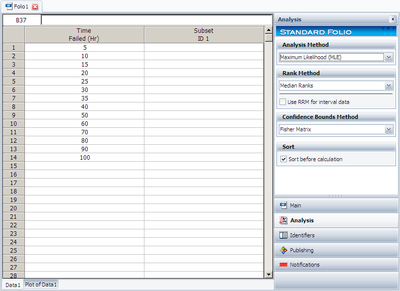
Using the data of Example 2 and assuming a normal distribution, estimate the parameters using the MLE method.
Solution
In this example we have non-grouped data without suspensions and without interval data. The partial derivatives of the normal log-likelihood function, [math]\displaystyle{ \Lambda , }[/math] are given by:
- [math]\displaystyle{ \begin{align}
\frac{\partial \Lambda }{\partial \mu }= & \frac{1}{{{\sigma }^{2}}}\underset{i=1}{\overset{14}{\mathop \sum }}\,({{t}_{i}}-\mu )=0 \\
\frac{\partial \Lambda }{\partial \sigma }= & \underset{i=1}{\overset{14}{\mathop \sum }}\,\left( \frac{{{t}_{i}}-\mu }{{{\sigma }^{3}}}-\frac{1}{\sigma } \right)=0
\end{align} }[/math]
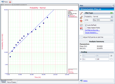
(The derivations of these equations are presented in Appendix.) Substituting the values of [math]\displaystyle{ {{t}_{i}} }[/math] and solving the above system simultaneously, we get [math]\displaystyle{ \widehat{\sigma }=29.58 }[/math] hours [math]\displaystyle{ , }[/math] [math]\displaystyle{ \widehat{\mu }=45 }[/math] hours [math]\displaystyle{ . }[/math]
The Fisher matrix is:
- [math]\displaystyle{ \left[ \begin{matrix}
\widehat{Var}\left( \widehat{\mu } \right)=62.5000 & {} & \widehat{Cov}\left( \widehat{\mu },\widehat{\sigma } \right)=0.0000 \\
{} & {} & {} \\
\widehat{Cov}\left( \widehat{\mu },\widehat{\sigma } \right)=0.0000 & {} & \widehat{Var}\left( \widehat{\sigma } \right)=31.2500 \\
\end{matrix} \right] }[/math]
Using Weibull++ , the MLE method can be selected from the Set Analysis page.
The plot of the solution for this example is shown next.

